Cross Correlation (CC)

Cross-correlation can be used to find where point $P$ in the reference_image can be found in the current_image.

There are many different implementations of cross-correlation. We discuss the varied implementations in Correlation Criteria. For now, it is sufficient to know only that cross-correlation is used to locate a point in a current image given a known location of that same point in a reference image. The current focus is to make the subordinate concepts underlying cross-correlation be well-defined and well-illustrated.

Let the kernel (also called a subset, filter, or convolution matrix) be a rectangular region of reference_image centered on $p_{0}$ , the vector that locates point $P$ from origin $O$ in the reference_image. The kernel is a small, distinctive patch of the reference image content that we want to locate within a subsequent image.

In the needle in a haystack idiom, the kernel is the needle, and the haystack is current_image. To keep the search tractable, we don't search the entire haystack — we constrain it to a search area (also called the area of interest (AOI), search window, or scanning zone). The search area is a subimage of the current_image, centered on a search_center, which is a guess of roughly where $P$ ended up, not the answer itself.

While there are techniques derived from macro deformation metrics that can provide a good first guess for the search_center, for simplicity, and since the deformations are small, we reuse $p_{0}$ itself as the search_center in this example.

Because the kernel and search area are themselves subimages of a larger image (see Subimage Generation), each subimage has its own local frame:

Let $K$ be the reference frame of the kernel subimage.
Let $S$ be the reference frame of the search area subimage.

reference_image, p0, current_image, and p1 are the same as in Single Point Motion:

from dictk.image import read, translate, PixelCoordinate

reference_image = read(path="checkerboard0.png")
p0 = PixelCoordinate(x=100, y=75)
dx, dy = -6, 8
current_image = translate(arr=reference_image, dx=dx, dy=dy)
p1 = PixelCoordinate(x=p0.x + dx, y=p0.y + dy)

Kernel

From reference_image, extract the kernel surrounding $p_{0}$ , with a 25-pixel margin on every side (50x50 total):

from dictk.plot import subimage_comparison_plot

kernel_margin = 25
kernel_origin = PixelCoordinate(x=p0.x - kernel_margin, y=p0.y - kernel_margin)
subimage_comparison_plot(
    image=reference_image,
    origin=kernel_origin,
    width=2 * kernel_margin,
    height=2 * kernel_margin,
    point=p0,
    point_color="orange",
    point_label="$P$",
    subimage_label="kernel",
    color="green",
    origin_label="$K$",
    source_origin_label="$O$",
    figsize=(6.4, 4.8),
    path="single_point_motion_kernel.png",
)

Saved: single_point_motion_kernel.png

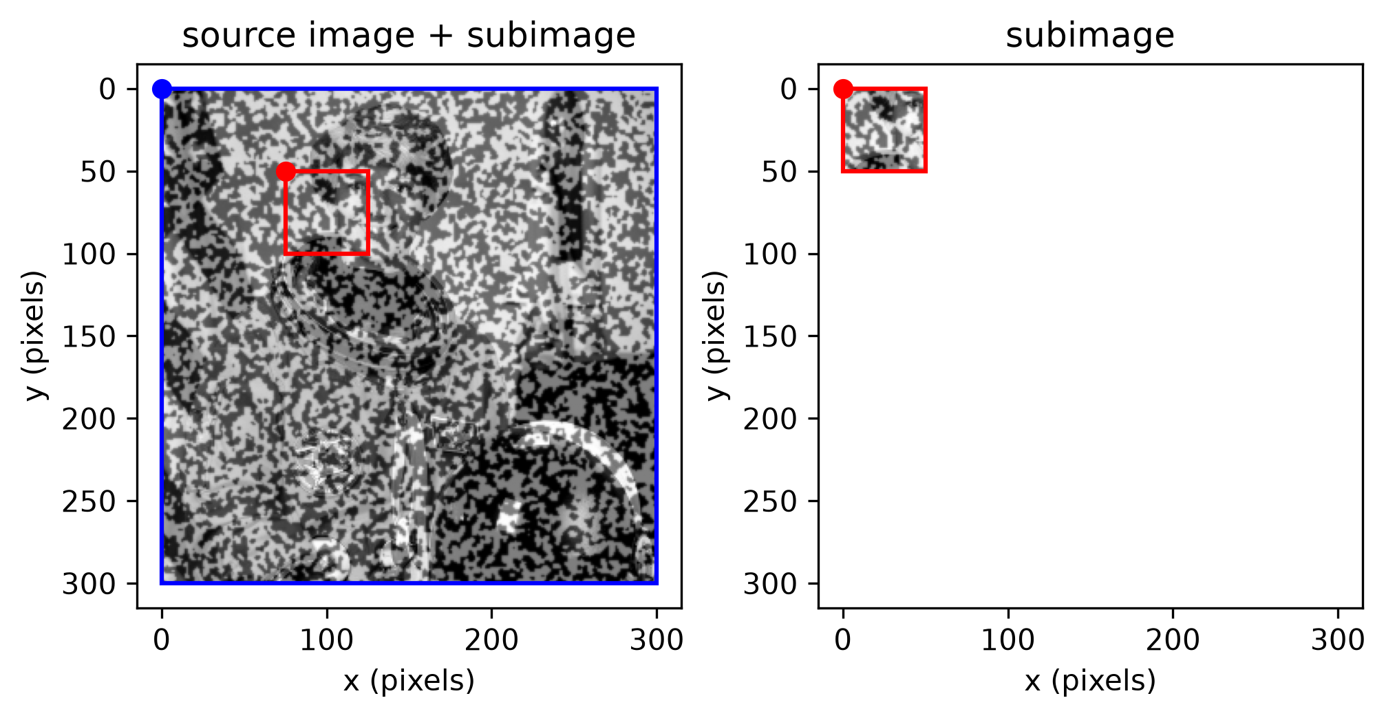
kernel placement in the reference image with point P marked by an orange dot, and the extracted kernel itself with point P marked by an orange dot — Left: the kernel (green box), a 50x50 region of `reference_image` centered on $p_{0}$ , with origin $r_{O K / F} = (75, 50)$ pixels (green dot); point $P$ itself is the orange dot at $p_{0} = (100, 75)$ . Right: the extracted kernel, in its own local reference frame $K$ ; the same point $P$ (orange dot) is now at $r_{K P / K} = (25, 25)$ pixels.

The kernel has its own local coordinate system $K$ , with origin $K$ at its top-left corner. Point $P$ 's position is the same in both frames, just expressed relative to a different origin:

$r_{OP / F} = r_{O K / F} + r_{K P / K}$

Since the kernel is centered on $p_{0}$ with a 25-pixel margin, $r_{K P / K} = (25, 25)$ pixels. Point $P$ always sits at (kernel_margin_width, kernel_margin_height) within the kernel's own frame, regardless of where the kernel came from in reference_image.

Search Area

From current_image, extract the search area surrounding search_center (here, $p_{0}$ again, since it is currently our best guess), with a 50-pixel margin on every side (100x100 total):

search_margin = 50
search_center = p0
search_origin = PixelCoordinate(
    x=search_center.x - search_margin, y=search_center.y - search_margin
)
subimage_comparison_plot(
    image=current_image,
    origin=search_origin,
    width=2 * search_margin,
    height=2 * search_margin,
    subimage_label="search area",
    origin_label="$S$",
    source_origin_label="$O$",
    figsize=(6.4, 4.8),
    path="single_point_motion_search.png",
)

Saved: single_point_motion_search.png

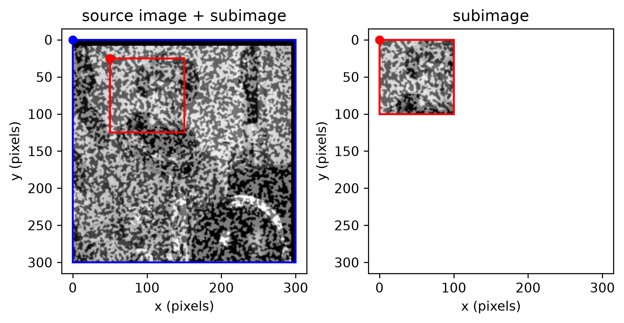
search area placement in the current image, and the extracted search area itself — Left: the search area (red box), a 100x100 region of `current_image` centered on `search_center`, with origin $r_{OS / F} = (50, 25)$ pixels (red dot); the source image's own origin is labeled $O$ , the search area's origin is labeled $S$ . Right: the extracted search area on its own, in its own local reference frame $S$ , with origin $S$ .

The search area likewise has its own local frame $S$ , origin $S$ at its top-left corner. The location of $P^{'}$ in the current_image is given by:

$r_{O P^{'} / F} = r_{OS / F} + r_{S P^{'} / S}$

The goal of the DIC process is to locate $P^{'}$ by solving for the quantity $r_{S P^{'} / S}$ . The location of $P^{'}$ in the search area's local frame is the single unknown; all other vectors are known.

Solution

The insight into the solution is to further decompose $r_{S P^{'} / S}$ into the sum of two additional vectors:

$r_{S P^{'} / S} = r_{S K / S} + r_{K P / K}$

The second term, $r_{K P / K}$ , is a known constant. The first term, $r_{S K / S}$ , is unknown and can be calculated using cross-correlation. When the kernel and search area subimages align, their cross-correlation is maximized. We find the maximum cross-correlation to determine $r_{S K / S}$ and thus calculate $r_{O P^{'} / F}$ .

$r_{O P^{'} / F} = r_{OS / F} + r_{S K / S} + r_{K P / K}$

This is exactly what dictk.translation.locate computes internally — via skimage.registration.phase_cross_correlation for $r_{S K / S}$ . The locate function returns $p_{1}$ directly (one does not assemble the vector chain manually).

phase_cross_correlation is a Fourier-domain computation — every locate call in this book takes that route under the hood, rather than sliding the kernel across the search area one position at a time. Correlation Criteria examines that Fourier-domain implementation in greater depth, alongside the spatial-domain CC, NCC, ZCC, and ZNCC criteria it complements.

Locating the Point

from dictk.translation import locate

found = locate(
    reference_image=reference_image,
    current_image=current_image,
    reference_point=p0,
    search_center=search_center,
    kernel_margin_width=kernel_margin,
    kernel_margin_height=kernel_margin,
    search_margin_width=search_margin,
    search_margin_height=search_margin,
)
print(f"found = {found}")
print(f"displacement = ({found.x - p0.x}, {found.y - p0.y})")

found = PixelCoordinate(x=94, y=83)
displacement = (-6, 8)

found matches the ground-truth $p_{1} = (94, 83)$ pixels from earlier, recovering the known displacement $δ p = (- 6, 8)$ pixels using only the two images and $p_{0}$ — exactly the information available for a real (not synthetically generated) image pair.

Visualizing the Solution

For illustration, we can back out $r_{S K / S}$ — the one quantity locate finds via cross-correlation, everything else here being known geometry — from found and the boxed equation above, and draw the full chain $r_{OS / F} + r_{S K / S} + r_{K P / K}$ on current_image:

from dictk.plot import point_plot, ArrowAnnotation, BoxAnnotation, PointAnnotation

r_sk = PixelCoordinate(
    x=found.x - search_origin.x - kernel_margin,
    y=found.y - search_origin.y - kernel_margin,
)
kernel_found_origin = PixelCoordinate(
    x=search_origin.x + r_sk.x, y=search_origin.y + r_sk.y
)
image_height, image_width = current_image.shape
point_plot(
    image=current_image,
    boxes=[
        BoxAnnotation(
            origin=PixelCoordinate(x=0, y=0),
            width=image_width,
            height=image_height,
            color="blue",
            label="source image",
        ),
        BoxAnnotation(
            origin=search_origin,
            width=2 * search_margin,
            height=2 * search_margin,
            color="red",
            label="search area",
        ),
        BoxAnnotation(
            origin=kernel_found_origin,
            width=2 * kernel_margin,
            height=2 * kernel_margin,
            color="green",
            label="kernel",
        ),
    ],
    points=[
        PointAnnotation(position=PixelCoordinate(x=0, y=0), label="$O$", color="blue"),
        PointAnnotation(position=search_origin, label="$S$", color="red"),
        PointAnnotation(position=kernel_found_origin, label="$K$", color="green"),
        PointAnnotation(position=found, label="$P$", color="black"),
    ],
    arrows=[
        ArrowAnnotation(
            tail=PixelCoordinate(x=0, y=0),
            head=found,
            color="cyan",
            label=r"$\boldsymbol{r}_{OP'/\mathcal{F}}$",
        ),
        ArrowAnnotation(
            tail=PixelCoordinate(x=0, y=0),
            head=search_origin,
            color="blue",
            label=r"$\boldsymbol{r}_{OS/\mathcal{F}}$: search area origin",
        ),
        ArrowAnnotation(
            tail=search_origin,
            head=kernel_found_origin,
            color="red",
            label=r"$\boldsymbol{r}_{SK/\mathcal{S}}$: kernel found in search area",
        ),
        ArrowAnnotation(
            tail=kernel_found_origin,
            head=found,
            color="green",
            label=r"$\boldsymbol{r}_{KP/\mathcal{K}}$: point within kernel",
        ),
    ],
    figsize=(6.4, 4.8),
    path="single_point_motion_solution_vectors.png",
)

Saved: single_point_motion_solution_vectors.png

chained vector solution: cyan shortcut arrow from origin directly to the found point, blue arrow from origin to search area origin, red arrow to the located kernel, green arrow to the found point, with a blue source-image box, a red search-area box, and a green kernel box drawn behind the arrows, and O, S, K, P labels drawn on top — The current configuration $p_{1}$ (tip of the cyan and green arrows) as the vector chain $r_{OS / F}$ (blue) $+ r_{S K / S}$ (red) $+ r_{K P / K}$ (green), equal to the direct shortcut $r_{O P^{'} / F}$ (cyan), drawn on `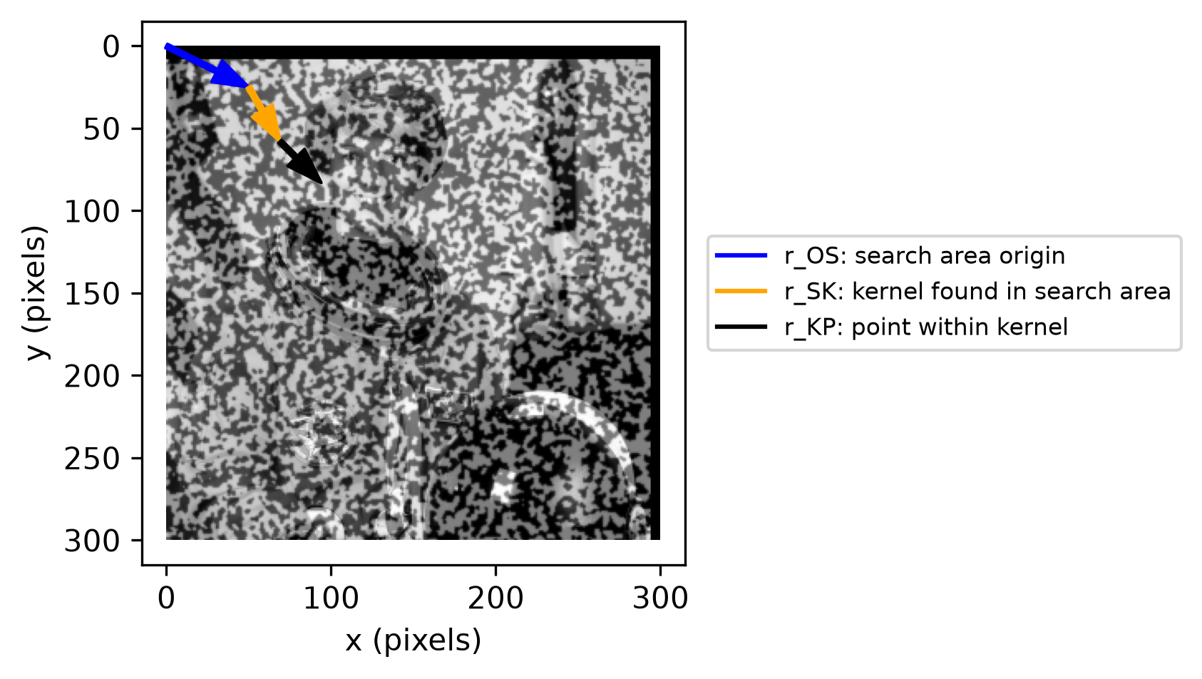current_image` — with the source image (blue box), search area (red box), and the kernel as found within it (green box) shown behind the arrows, each origin labeled: $O$ , $S$ , $K$ , and the found point $P$ .

vector, value	description
$r_{OS / F} = (50, 25)$ +	origin of the search area (blue arrow)
$r_{S K / S} = (19, 33)$ +	kernel located within the search area, from cross-correlation (red arrow)
$r_{K P / K} = (25, 25)$ =	point's fixed position within the kernel (green arrow)
$r_{O P^{'} / F} = (94, 83)$	current position $p_{1}$ , matching `found` above (cyan arrow)

NOTE: Cross-correlation may be conceptualized as the sliding dot product of pixel values from the kernel with pixel values from the search area. In this discussion we have described sliding the kernel across a stationary search area. The reverse, sliding the search area across a stationary kernel, is conceptually different but mathematically identical. Both approaches yield the same result: $r_{S K / S}$ , which locates the kernel frame in the search area frame.

Next: Correlation Criteria defines the four cross-correlation formulas and explains the Fourier-domain route locate actually takes, and Correlation Visualization visualizes each of them on this same kernel and search area.