Keyboard shortcuts

Press or to navigate between chapters

Press S or / to search in the book

Press ? to show this help

Press Esc to hide this help

Single Point Motion

Let origin be located at the top, left of the image. We attach reference frame to the origin, with the -axis running left-to-right and the -axis running top-to-bottom — the same pixel reference frame used throughout this guide (see Subimage Generation).

Consider a single point , fixed to a physical location on the object being imaged. In the reference image , this point is at a known pixel location pixels — we use the shorthand for this reference configuration. Between the reference image and a later current image , the object (and therefore ) may move. Finding 's new location — its current configuration — in , given only , is the problem this page works through, using dictk.translation.locate.

Reference Configuration

The examples below reuse astronaut0, the speckle pattern combined with the astronaut photo introduced in Image Generation and used again in Subimage Generation — here called reference_image, matching locate's own parameter name:

import dictk
from dictk.image import combine, PixelCoordinate, point_plot, ArrowAnnotation

speckle = dictk.rosta(width=300, height=300, density=0.5)
photo = dictk.astronaut(width=300, height=300)
reference_image = combine(a=speckle, b=photo)

p0 = PixelCoordinate(x=100, y=75)
point_plot(
    image=reference_image,
    arrows=[
        ArrowAnnotation(
            tail=PixelCoordinate(x=0, y=0), head=p0, color="gold", label="p0"
        )
    ],
    path="single_point_motion_p0.png",
)
Saved: single_point_motion_p0.png
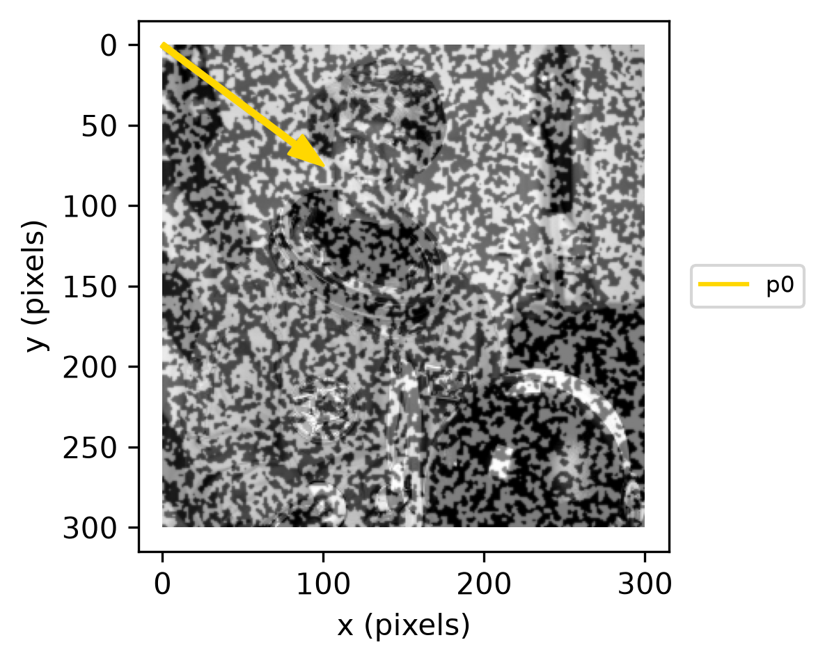
reference image with reference configuration p0 marked by a gold arrow from the origin
Reference image and reference configuration (gold arrow) pixels.

Current Configuration and Displacement

For this page, the current image is generated with dictk.image.translate (see Image Transformation): every pixel of reference_image shifts by the same (dx, dy), a rigid body translation — one of the simplest deformation categories (see Image Transformation for the full set). Because the whole image moves together, point 's new location follows directly:

from dictk.image import translate

current_image = translate(arr=reference_image, dx=-6, dy=8)
p1 = PixelCoordinate(x=p0.x - 6, y=p0.y + 8)  # ground truth, known here by construction

We define the displacement of the point as the relative motion between the reference configuration and the current configuration , such that

so with and ,

point_plot(
    image=current_image,
    arrows=[
        ArrowAnnotation(
            tail=PixelCoordinate(x=0, y=0), head=p1, color="cyan", label="p1"
        ),
        ArrowAnnotation(tail=p0, head=p1, color="magenta", label="displacement"),
    ],
    path="single_point_motion_p1_displacement.png",
)
Saved: single_point_motion_p1_displacement.png
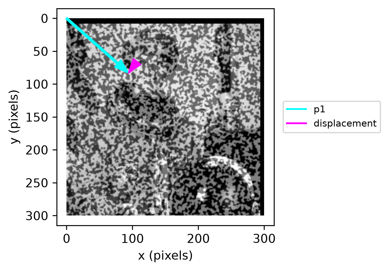
current image with current configuration p1 marked by a cyan arrow from the origin, and displacement marked by a magenta arrow from p0 to p1
Current image with current configuration (cyan arrow) pixels, and displacement (magenta arrow) pixels.

Of course, p1 above was only known in advance because we generated current_image ourselves with a known translate. In practice — a real pair of DIC images — is exactly what's unknown and needs to be found. The rest of this page finds it using only reference_image, current_image, and , the same information available in the real case, to demonstrate that locate recovers it correctly.

Cross-Correlation

We use cross-correlation to find where point moved to. Let the kernel — also called a subset, filter, or convolution matrix — be a rectangular region of reference_image centered on . The kernel is a small, distinctive patch of image content that we want to locate within a subsequent image.

In the needle in a haystack idiom, the kernel is the needle, and the haystack is current_image. To keep the search tractable, we don't search the entire haystack — we constrain it to a search area (also called a search window, scanning zone, or area of interest (AOI)), a larger rectangular region of current_image centered on a search_center — a guess of roughly where ended up, not the answer itself. Here, with no better guess available, we reuse itself as search_center.

Kernel

From reference_image, extract the kernel surrounding , with a 25-pixel margin on every side (50x50 total):

from dictk.image import subimage_comparison_plot

kernel_margin = 25
kernel_origin = PixelCoordinate(x=p0.x - kernel_margin, y=p0.y - kernel_margin)
subimage_comparison_plot(
    image=reference_image,
    origin=kernel_origin,
    width=2 * kernel_margin,
    height=2 * kernel_margin,
    path="single_point_motion_kernel.png",
)
Saved: single_point_motion_kernel.png
kernel placement in the reference image, and the extracted kernel itself
Left: the kernel (red box), a 50x50 region of reference_image centered on , with origin pixels (red 'o'). Right: the extracted kernel on its own, in its own local reference frame .

The kernel has its own local coordinate system , with origin at its top-left corner. Point 's position is the same in both frames, just expressed relative to a different origin:

Since the kernel is centered on with a 25-pixel margin, pixels — point always sits at (kernel_margin_width, kernel_margin_height) within the kernel's own frame, regardless of where the kernel came from in reference_image.

Search Area

From current_image, extract the search area surrounding search_center (here, again), with a 50-pixel margin on every side (100x100 total):

search_margin = 50
search_center = p0
search_origin = PixelCoordinate(
    x=search_center.x - search_margin, y=search_center.y - search_margin
)
subimage_comparison_plot(
    image=current_image,
    origin=search_origin,
    width=2 * search_margin,
    height=2 * search_margin,
    path="single_point_motion_search.png",
)
Saved: single_point_motion_search.png
search area placement in the current image, and the extracted search area itself
Left: the search area (red box), a 100x100 region of current_image centered on search_center, with origin pixels (red 'o'). Right: the extracted search area on its own, in its own local reference frame .

The search area likewise has its own local frame , origin at its top-left corner:

where is point 's current position — what we're trying to find. , its position within the search area's local frame, is still unknown at this point.

Solution

Cross-correlation fixes the search area and finds where the kernel's content best aligns within it — the kernel's own origin , located relative to the search area's origin : . Once is located, 's position within the search area follows from the same kernel-local offset found above:

Substituting into the search area's equation gives the full chain from the shared origin to :

This is exactly what dictk.translation.locate computes internally — via skimage.registration.phase_cross_correlation for — so as a caller, you don't assemble this chain by hand; locate returns directly.

Locating the Point

from dictk.translation import locate

found = locate(
    reference_image=reference_image,
    current_image=current_image,
    reference_point=p0,
    search_center=search_center,
    kernel_margin_width=kernel_margin,
    kernel_margin_height=kernel_margin,
    search_margin_width=search_margin,
    search_margin_height=search_margin,
)
print(f"found = {found}")
print(f"displacement = ({found.x - p0.x}, {found.y - p0.y})")
found = PixelCoordinate(x=94, y=83)
displacement = (-6, 8)

found matches the ground-truth pixels from earlier, recovering the known displacement pixels using only the two images and — exactly the information available for a real (not synthetically generated) image pair.

Visualizing the Solution

For illustration, we can back out — the one quantity locate finds via cross-correlation, everything else here being known geometry — from found and the boxed equation above, and draw the full chain on current_image:

r_sk = PixelCoordinate(
    x=found.x - search_origin.x - kernel_margin,
    y=found.y - search_origin.y - kernel_margin,
)
point_plot(
    image=current_image,
    arrows=[
        ArrowAnnotation(
            tail=PixelCoordinate(x=0, y=0),
            head=search_origin,
            color="blue",
            label="r_OS: search area origin",
        ),
        ArrowAnnotation(
            tail=search_origin,
            head=PixelCoordinate(x=search_origin.x + r_sk.x, y=search_origin.y + r_sk.y),
            color="orange",
            label="r_SK: kernel found in search area",
        ),
        ArrowAnnotation(
            tail=PixelCoordinate(x=search_origin.x + r_sk.x, y=search_origin.y + r_sk.y),
            head=found,
            color="black",
            label="r_KP: point within kernel",
        ),
    ],
    path="single_point_motion_solution_vectors.png",
)
Saved: single_point_motion_solution_vectors.png
chained vector solution: blue arrow from origin to search area origin, orange arrow to the located kernel, black arrow to the found point
The current configuration (tip of the black arrow) as the vector chain (blue) (orange) (black), drawn on current_image.
vector, valuedescription
+origin of the search area (blue arrow)
+kernel located within the search area, from cross-correlation (orange arrow)
=point's fixed position within the kernel (black arrow)
current position , matching found above