Subimage Generation
Now we consider extracting a subimage from a subject image. A subimage is a useful precursor to image computation: narrowing the data down to a region of interest makes the computation more efficient than considering the full image.
Reference Frames
When we have just a single image, we have a single, trivial reference
frame : origin (blue dot) at the top-left corner, with
the -axis (red) running left-to-right and the -axis (green)
running top-to-bottom. origin, and every pixel coordinate on this
page, is expressed in this frame — one that's always implicitly
present, even in the left panel below where nothing is drawn to show
it. astronaut0 here is the same reference image created in Image
Generation:
from dictk.image import read
from dictk.plot import reference_frame_plot

astronaut0 = read(path="astronaut0.png")
reference_frame_plot(image=astronaut0, path="reference_frame.png")
Saved: reference_frame.png
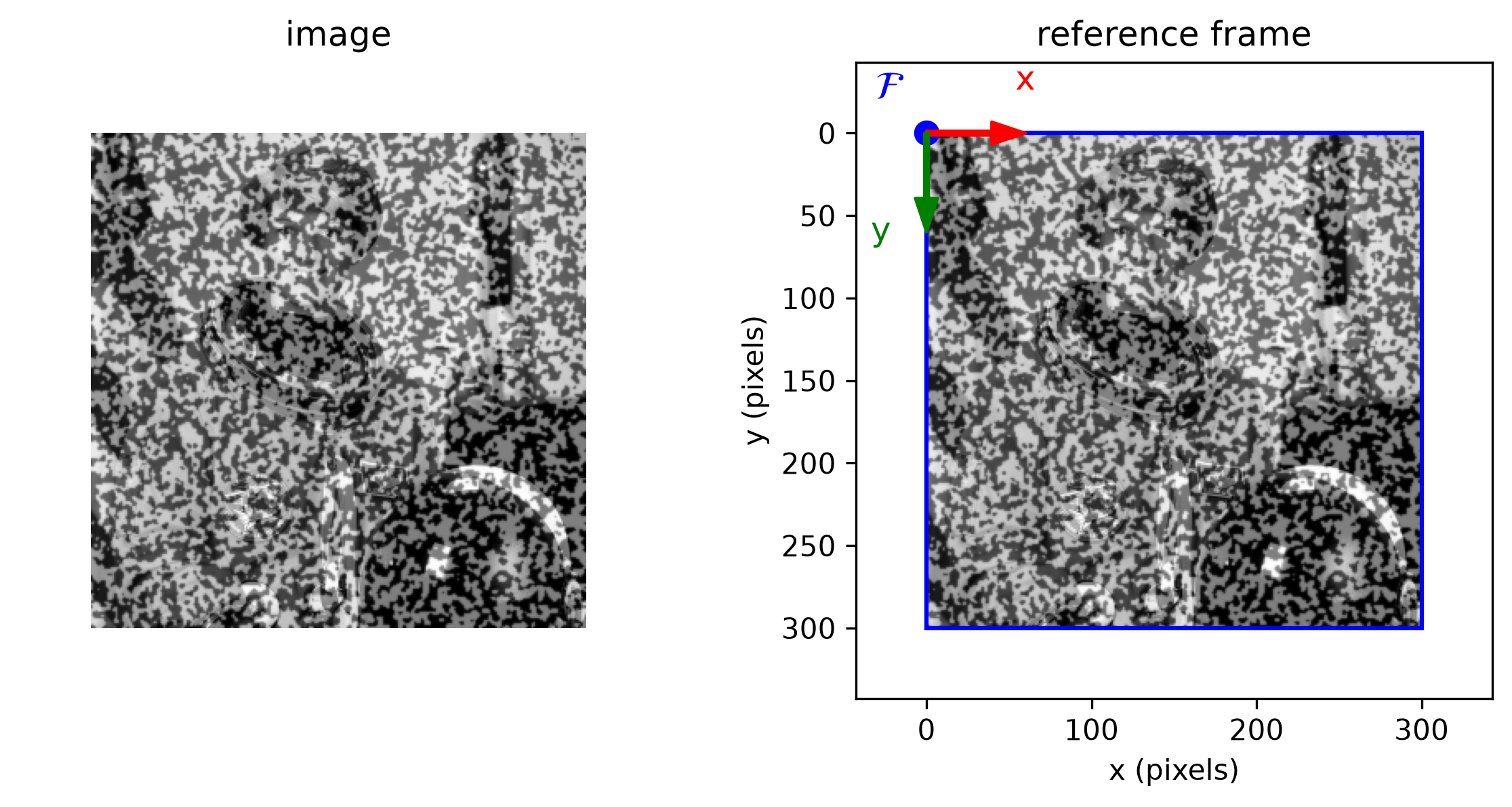
astronaut0 (300x300 pixels) alone. Right: the same image with its reference frame made explicit and labeled near the origin — origin (blue dot) at the top-left corner, -axis (red), and -axis (green), used throughout this page.When we extract a subimage from an image, it is useful to be explicit about reference frames: the subimage has its own frame , located within the image's frame . The Python API section below demonstrates this concept.
Python API
dictk.image.subimage extracts a
rectangular crop from a source image: a width x height region whose
top-left corner sits at origin. origin may place the requested
region partially or completely outside the source image — rather than
raising an error, subimage fills whatever doesn't overlap with black
(zero) pixels, so the result is always a well-formed height x width
array. This is the building block later tutorials use to pull a kernel
or search area out of a larger reference/current image pair around a
point of interest.
dictk.image.PixelCoordinate
is a simple (x, y) NamedTuple used for origin.
dictk.image.subimage itself
returns the cropped array directly, with no file written.
The examples below use
subimage_comparison_plot,
which saves a two-panel figure: the left panel shows where the region
falls relative to the source image (blue/red boxes), and the right panel
shows the extracted result on its own, in its own local frame
— sharing the same axis limits as the left panel so the
two red boxes render at matching scale. It's built from two smaller
single-panel functions, also available individually:
subimage_bounds_plot
(the left panel alone) and
subimage_plot (the right
panel alone, but zoomed to the subimage's own size rather than sharing
the source image's scale).
Square, fully inside
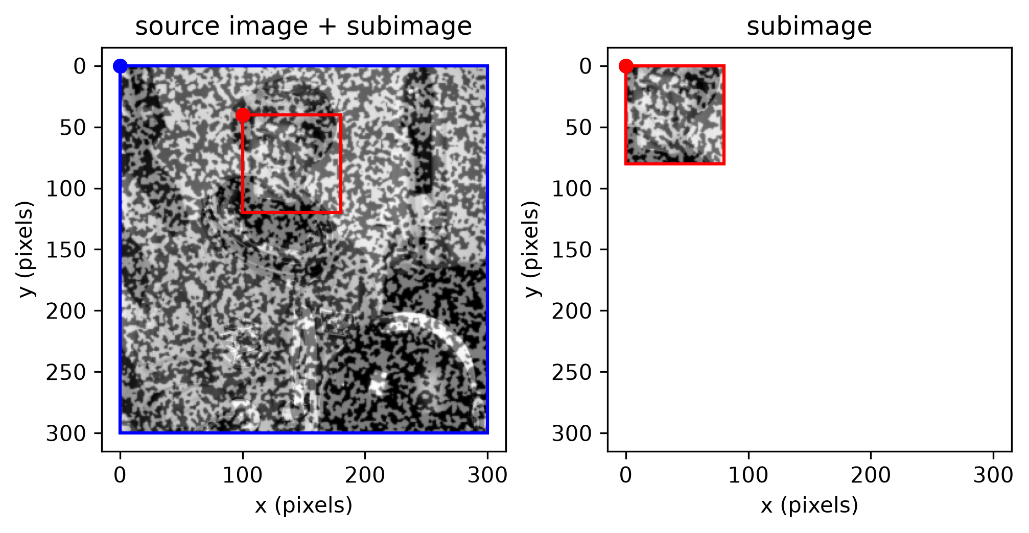
An 80x80 square region entirely within astronaut0's 300x300 bounds.
subimage_comparison_plot
draws both panels side by side, sharing the same axis limits, so the
red box in the right panel renders at identical scale to the one on the
left.
from dictk.image import PixelCoordinate
from dictk.plot import subimage_comparison_plot

origin = PixelCoordinate(x=100, y=40)
subimage_comparison_plot(image=astronaut0, origin=origin, width=80, height=80, path="subimage_comparison_80w_by_80h_at_100_40.png")
Saved: subimage_comparison_80w_by_80h_at_100_40.png
Rectangle, fully inside
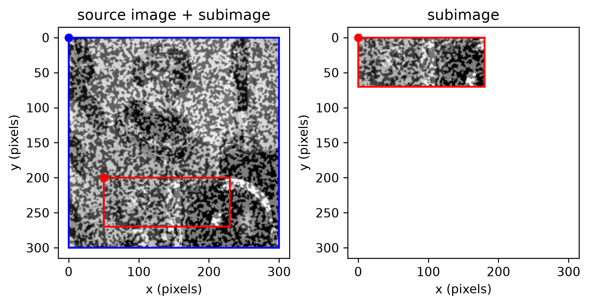
A 180x70 region — wider than it is tall — also entirely within the source image bounds:
from dictk.image import PixelCoordinate
from dictk.plot import subimage_comparison_plot

origin = PixelCoordinate(x=50, y=200)
subimage_comparison_plot(image=astronaut0, origin=origin, width=180, height=70, path="subimage_comparison_180w_by_70h_at_50_200.png")
Saved: subimage_comparison_180w_by_70h_at_50_200.png
Partially outside
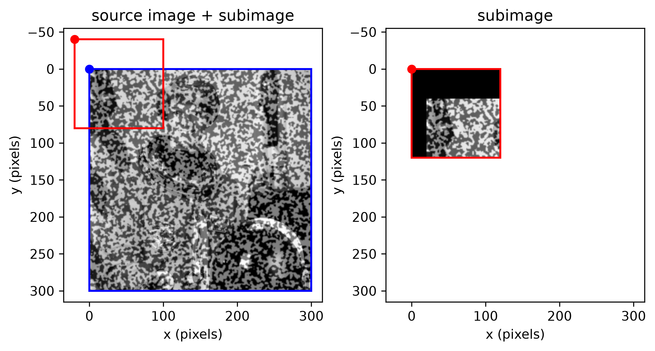
A 120x120 region with a negative origin, straddling the source image's
top-left corner. subimage fills the part of the region above and to
the left of the source with black:
from dictk.image import PixelCoordinate
from dictk.plot import subimage_comparison_plot

origin = PixelCoordinate(x=-20, y=-40)
subimage_comparison_plot(image=astronaut0, origin=origin, width=120, height=120, path="subimage_comparison_120w_by_120h_at_-20_-40.png")
Saved: subimage_comparison_120w_by_120h_at_-20_-40.png
astronaut0.Completely outside
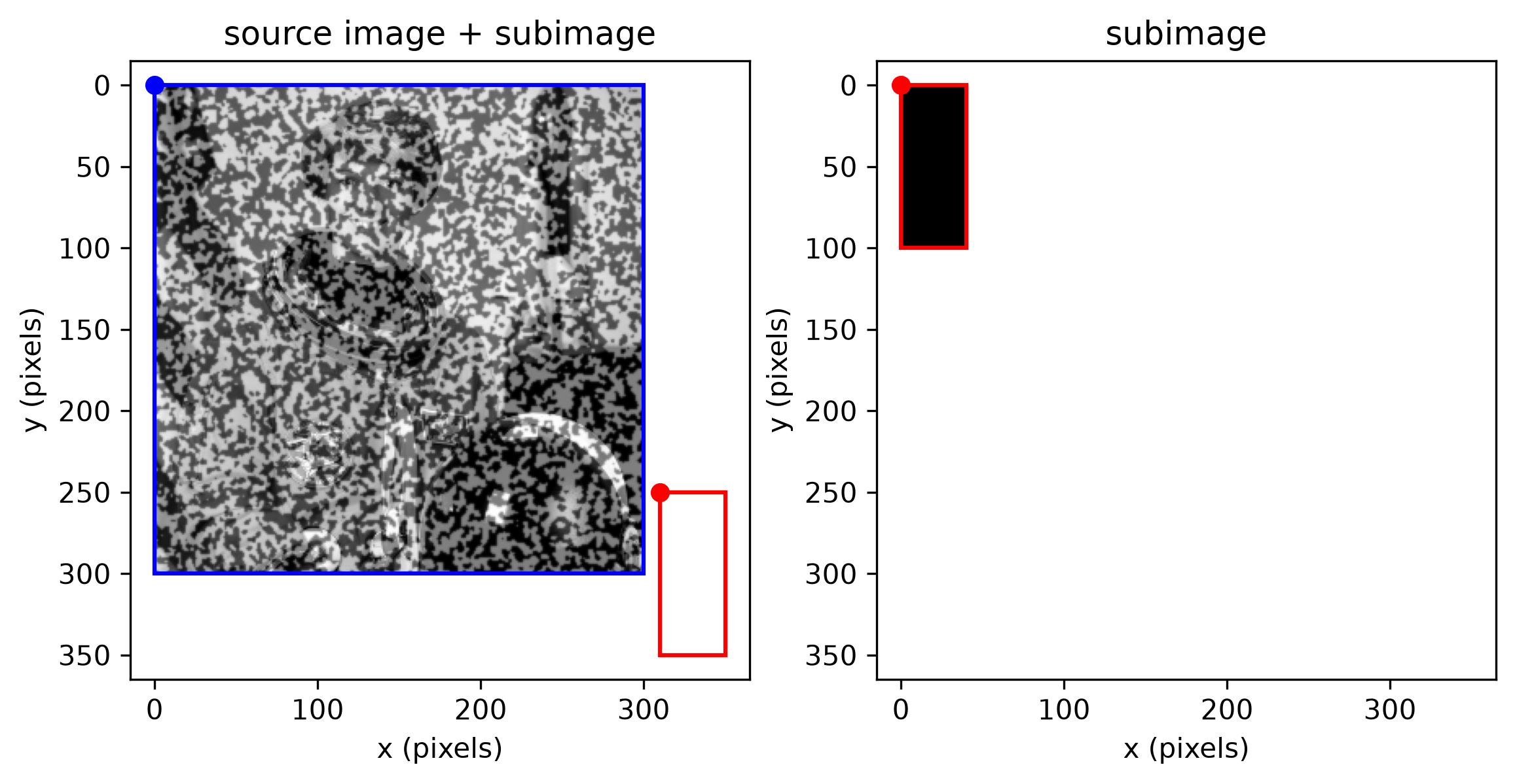
A 40x100 region entirely beyond the source image's bounds — its x-range (310 to 350) shares no pixels with the source's (0 to 300), so there is no overlap at all and the result is entirely black:
from dictk.image import PixelCoordinate
from dictk.plot import subimage_comparison_plot

origin = PixelCoordinate(x=310, y=250)
subimage_comparison_plot(image=astronaut0, origin=origin, width=40, height=100, path="subimage_comparison_40w_by_100h_at_310_250.png")
Saved: subimage_comparison_40w_by_100h_at_310_250.png
astronaut0.