Correlation Visualization

This page visualizes each of the four spatial-domain correlation criteria from Correlation Criteria — CC, NCC, ZCC, and ZNCC — one at a time, in a four-panel composite reproducing a reference composite-figure layout used in prior DIC tooling, via dictk.plot.spatial_correlation_quadrant_plot: the search area with the found kernel marked (Fixed Image), the kernel itself zero-padded to the search area's shape (Moving Image), the full correlation surface, and a zoomed Solution Vicinity around its peak — closer to how a single registration result is typically inspected in practice than a side-by-side comparison of criteria.

reference_image, p0, current_image, kernel_margin, search_margin, kernel, and search are the same as in Cross Correlation (CC):

from dictk.image import read, translate, PixelCoordinate, subimage

reference_image = read(path="checkerboard0.png")
p0 = PixelCoordinate(x=100, y=75)
current_image = translate(arr=reference_image, dx=-6, dy=8)

kernel_margin = 25
kernel = subimage(
    image=reference_image,
    origin=PixelCoordinate(x=p0.x - kernel_margin, y=p0.y - kernel_margin),
    width=2 * kernel_margin,
    height=2 * kernel_margin,
)

search_margin = 50
search_center = p0
search = subimage(
    image=current_image,
    origin=PixelCoordinate(
        x=search_center.x - search_margin, y=search_center.y - search_margin
    ),
    width=2 * search_margin,
    height=2 * search_margin,
)

The Fixed Image panel below plots the search area in its own pixel frame $S$ , with a yellow dashed box marking where the kernel was found and red/green dashed guide lines through that box's origin — the same $r_{S K / S}$ quantity Cross Correlation (CC) solves for by hand. The Correlation Surface panel plots that same quantity as candidate offset $(Δ x, Δ y)$ and marks the peak with a red circle of radius vicinity_margin (4 pixels by default) — exactly the region the Solution Vicinity panel zooms into, so the same circle reappears there too, now clipped by that panel's own edges.

Cross-Correlation (CC)

from dictk.correlation import cc
from dictk.plot import spatial_correlation_quadrant_plot

spatial_correlation_quadrant_plot(
    kernel=kernel,
    search=search,
    correlation_surface=cc(kernel=kernel, search=search),
    title="Cross-Correlation (CC)",
    path="correlation_visualization_cc.png",
)

Saved: correlation_visualization_cc.png

four-panel composite: fixed image with the found kernel boxed in yellow and red/green guide lines, the zero-padded moving image, the CC correlation surface, and a zoomed solution vicinity around its peak — CC's quadrant composite. The Correlation Surface panel is 51×51 — search's 100×100 minus kernel's 50×50, plus one in each dimension — since a value is only defined where the 50×50 kernel fits entirely inside the 100×100 search area ("valid" positions, no wraparound). checkerboard0's tiled pattern repeats every ~25 pixels, so that panel shows more than one strong local peak within its own (smaller, "valid") range — CC has no way to prefer the true one over its look-alikes beyond raw magnitude, unlike the normalized criteria below. 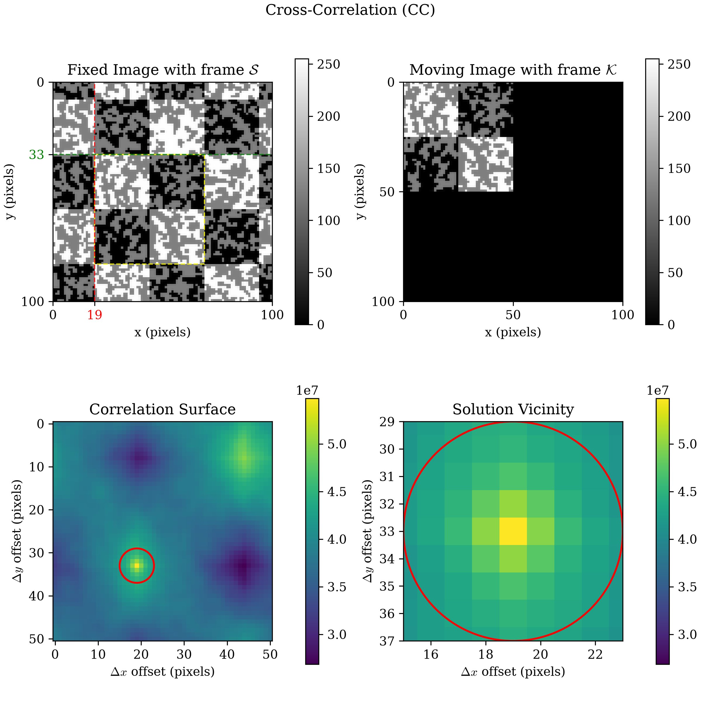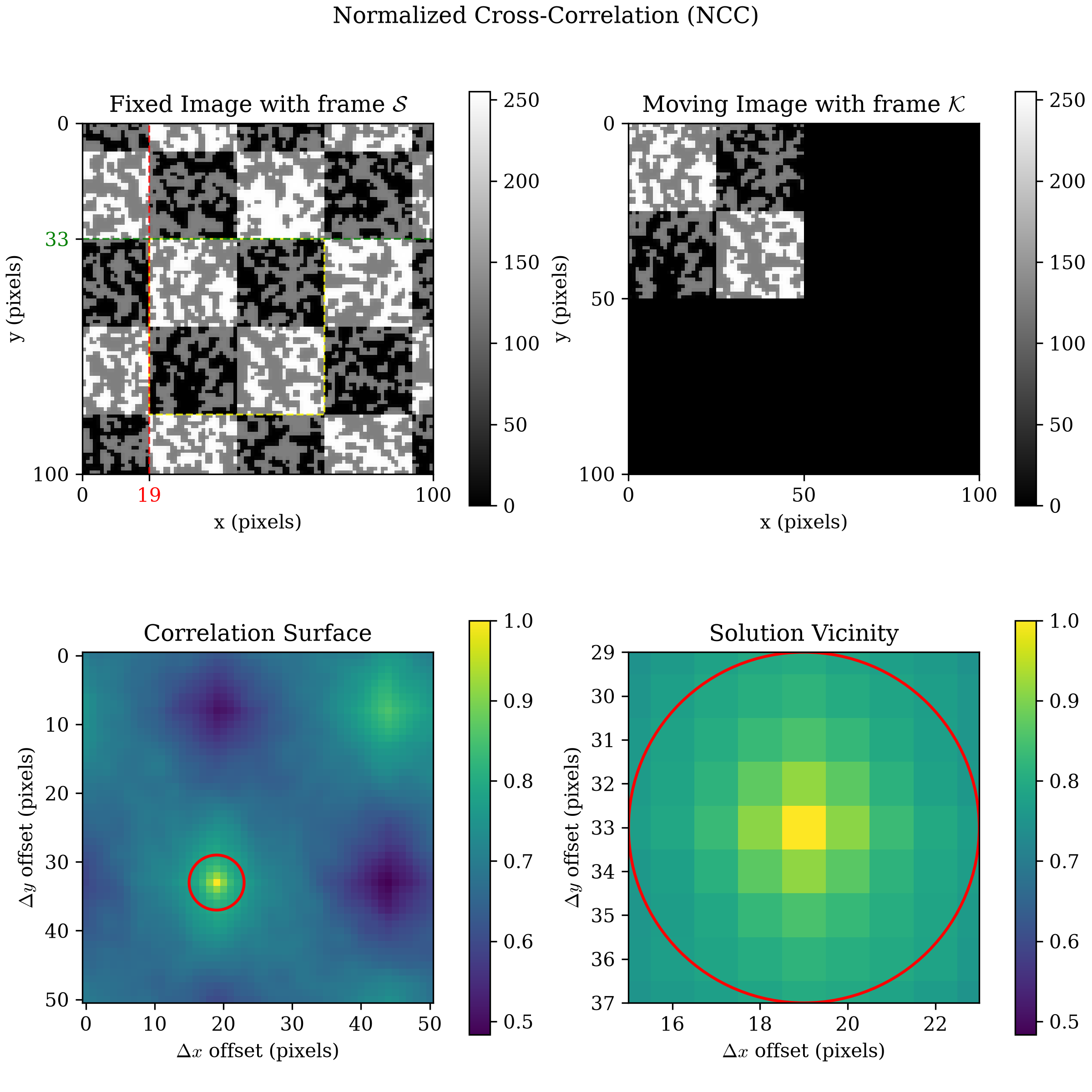The correct one, boxed in yellow in the Fixed Image panel, sits at $r_{S K / S} = (19, 33)$ pixels — matching the value already found by `locate` in Cross Correlation (CC).

Normalized Cross-Correlation (NCC)

from dictk.correlation import ncc

spatial_correlation_quadrant_plot(
    kernel=kernel,
    search=search,
    correlation_surface=ncc(kernel=kernel, search=search),
    title="Normalized Cross-Correlation (NCC)",
    path="correlation_visualization_ncc.png",
)

Saved: correlation_visualization_ncc.png

four-panel composite for NCC: fixed image with the found kernel boxed in yellow and red/green guide lines, the zero-padded moving image, the NCC correlation surface, and a zoomed solution vicinity around its peak — NCC's quadrant composite, bounded to $[- 1, 1]$ by construction — visible in the colorbar range compared to CC's arbitrary raw units above. Its Correlation Surface panel is the same 51×51 "valid"-positions-only shape as CC's above. Its peak still lands at $r_{S K / S} = (19, 33)$ pixels, matching the value already found by `locate` in Cross Correlation (CC).

Zero-mean Cross-Correlation (ZCC)

from dictk.correlation import zcc

spatial_correlation_quadrant_plot(
    kernel=kernel,
    search=search,
    correlation_surface=zcc(kernel=kernel, search=search),
    title="Zero-mean Cross-Correlation (ZCC)",
    path="correlation_visualization_zcc.png",
)

Saved: correlation_visualization_zcc.png

four-panel composite for ZCC: fixed image with the found kernel boxed in yellow and red/green guide lines, the zero-padded moving image, the ZCC correlation surface, and a zoomed solution vicinity around its peak — ZCC's quadrant composite — raw units like CC's (mean-subtraction alone doesn't bound the range), but brightness-invariant per Correlation Criteria's table. Its Correlation Surface panel is the same 51×51 "valid"-positions-only shape as CC's and NCC's above. 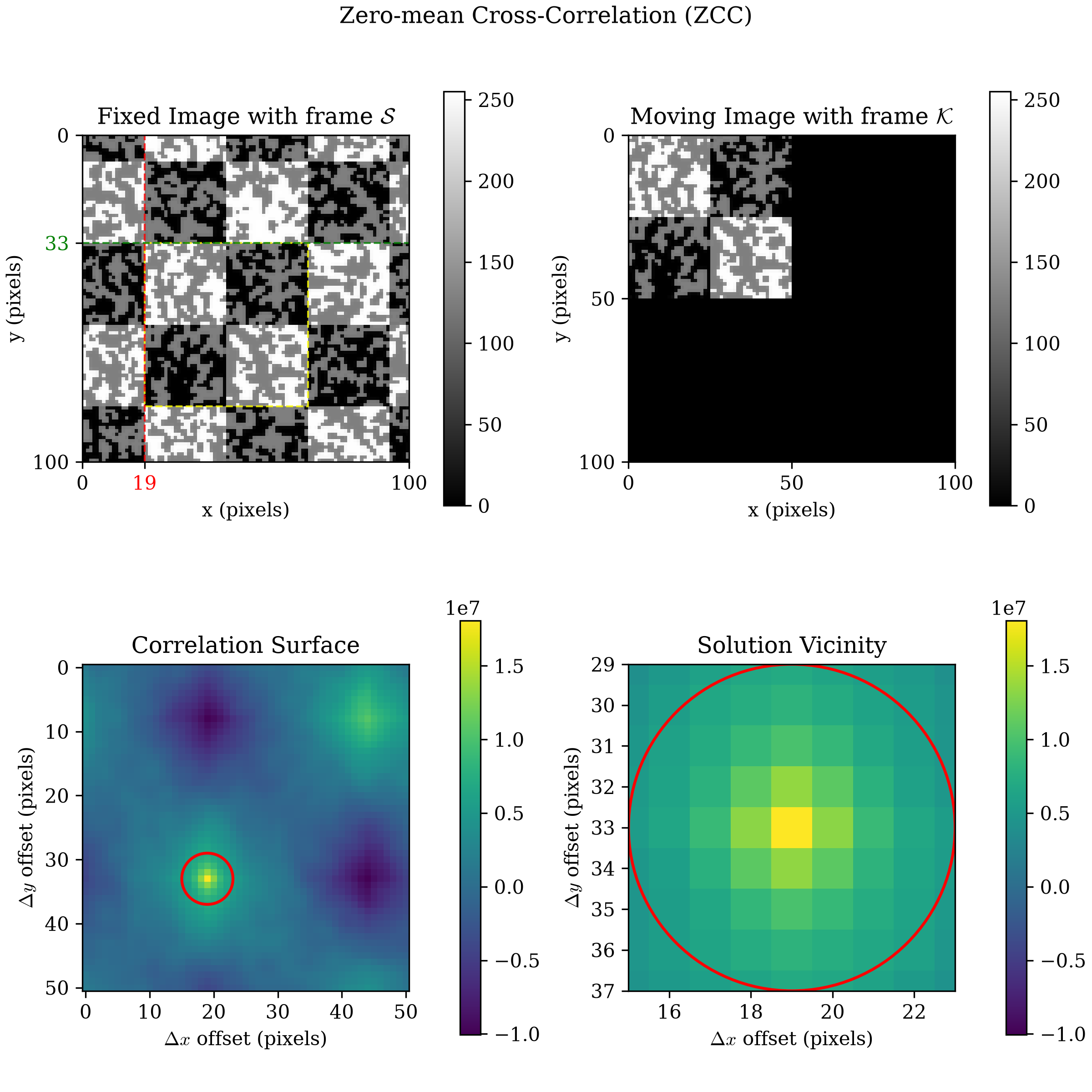Same peak, $r_{S K / S} = (19, 33)$ pixels, as `locate` already found in Cross Correlation (CC).

Zero-mean Normalized Cross-Correlation (ZNCC)

from dictk.correlation import zncc

spatial_correlation_quadrant_plot(
    kernel=kernel,
    search=search,
    correlation_surface=zncc(kernel=kernel, search=search),
    title="Zero-mean Normalized Cross-Correlation (ZNCC)",
    path="correlation_visualization_zncc.png",
)

Saved: correlation_visualization_zncc.png

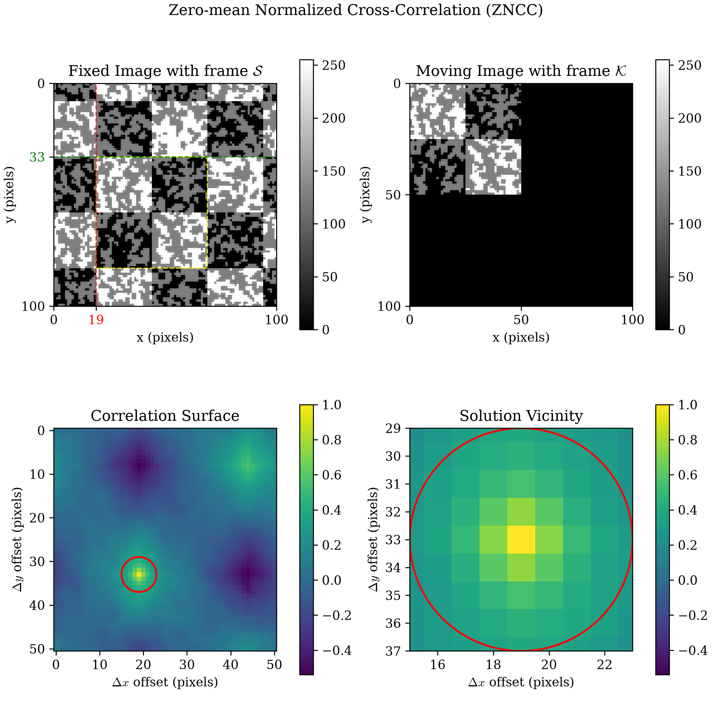
four-panel composite for ZNCC: fixed image with the found kernel boxed in yellow and red/green guide lines, the zero-padded moving image, the ZNCC correlation surface, and a zoomed solution vicinity around its peak — ZNCC's quadrant composite — both bounded to $[- 1, 1]$ and invariant to brightness and contrast, which is why `dictk.translation.locate`'s own underlying `skimage.registration.phase_cross_correlation` call is built on the same combination (see Correlation Criteria). Its Correlation Surface panel is likewise 51×51, "valid" positions only. Peak still at $r_{S K / S} = (19, 33)$ pixels, matching `locate`'s own result in Cross Correlation (CC).

All four land on the same peak, $r_{S K / S} = (19, 33)$ pixels, since kernel and search here share identical brightness and contrast (both come from checkerboard0.png, only translated). What differs between the four is what each panel's colorbar reveals about how safely that peak can be trusted once brightness or contrast do differ, as Correlation Criteria covers in detail.

Phase Correlation

Every panel above comes from a spatial-domain criterion — dictk.correlation's cc/ncc/zcc/ zncc, sliding kernel over search one window at a time. There's a second way to get an equivalent answer: all at once, in the Fourier domain, via dictk.correlation.phase_correlation — the same computation dictk.translation.locate already runs internally via skimage.registration.phase_cross_correlation. Unlike its spatial-domain siblings, there's only one Fourier-domain flavor here, so phase_correlation_quadrant_plot takes kernel/search directly rather than a pre-computed surface — no method to choose, nothing to compute beforehand. It does, however, take an optional windowing parameter (see Windowing): the three subsections below run this same kernel/search pair through no windowing, Hann windowing, and Hamming windowing in turn, so the effect is directly comparable rather than just described.

No Windowing (default)

windowing defaults to None, applying no tapering — this reproduces exactly what every earlier page in this book that calls phase_correlation/locate already does.

from dictk.plot import phase_correlation_quadrant_plot

phase_correlation_quadrant_plot(
    kernel=kernel,
    search=search,
    title="Phase Correlation (No Windowing)",
    path="correlation_visualization_phase_none.png",
)

Saved: correlation_visualization_phase_none.png

four-panel composite for phase correlation with no windowing: fixed image with the found kernel boxed in yellow and red/green guide lines, the zero-padded moving image, a correlation surface that is essentially flat except for one sharp isolated peak, and a zoomed solution vicinity around that peak — Phase correlation's quadrant composite, no windowing. 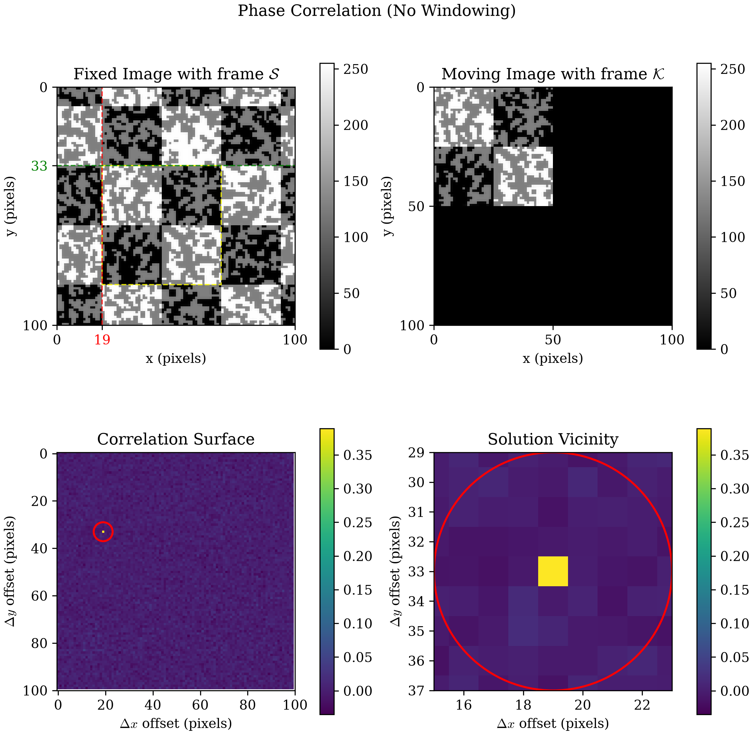Its Correlation Surface panel is a different size than the four above: 100×100, matching `search` itself, since `kernel` is zero-padded up to `search`'s shape before the FFT rather than restricted to "valid" positions — every candidate offset, including circular wraparound ones, gets a value. Same peak, $r_{S K / S} = (19, 33)$ pixels — matching the value already found by `locate` in Cross Correlation (CC) — as every criterion above, but the correlation-surface panel looks nothing like them: essentially flat/uniform everywhere except one crisp, isolated cell, rather than the broader, multi-peaked terrain CC/NCC/ZCC/ZNCC show on this same tiled `checkerboard0.png`.

Hann Windowing

from dictk.correlation import WindowingMethod

phase_correlation_quadrant_plot(
    kernel=kernel,
    search=search,
    windowing=WindowingMethod.HANN,
    title="Phase Correlation (Hann Windowing)",
    path="correlation_visualization_phase_hann.png",
)

Saved: correlation_visualization_phase_hann.png

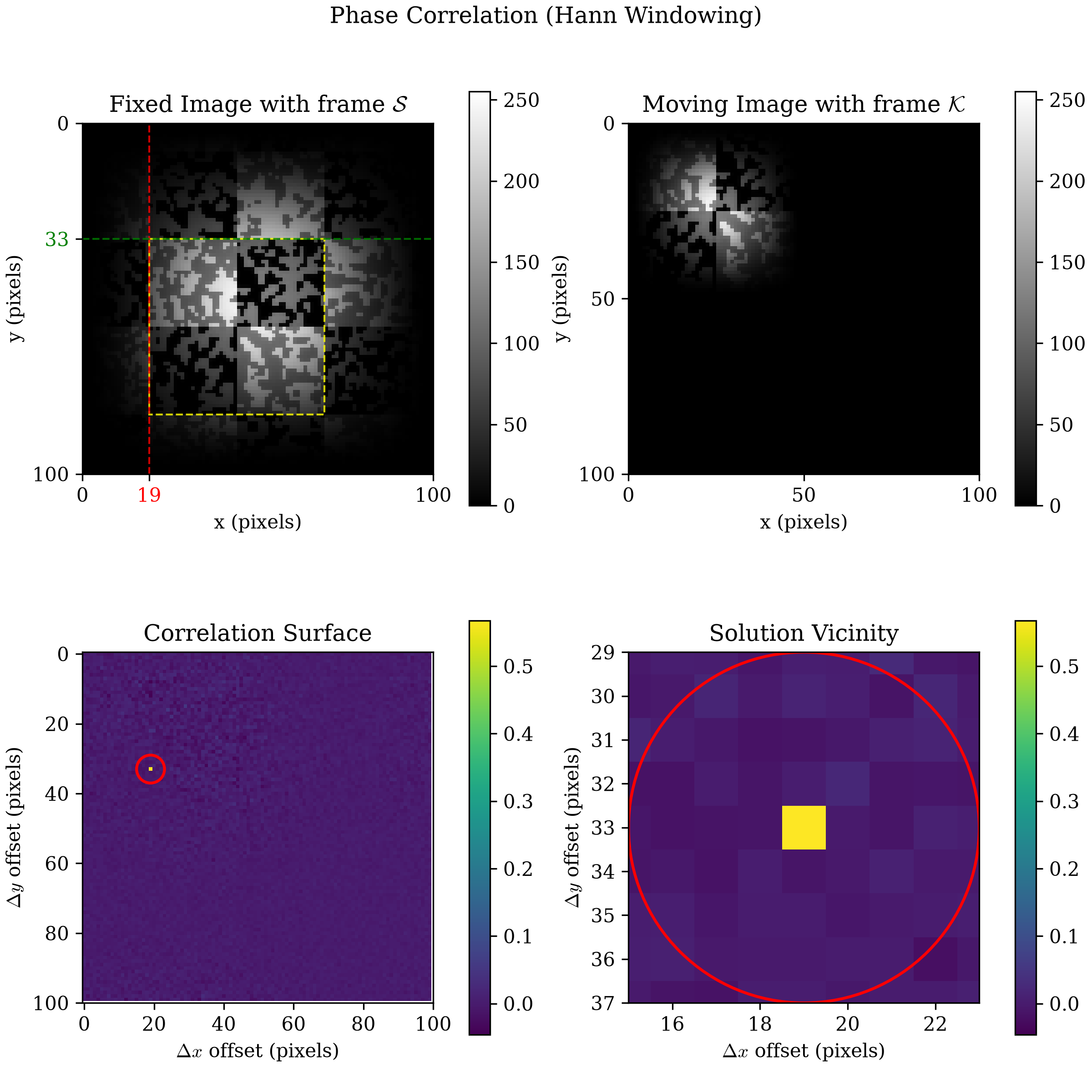
four-panel composite for phase correlation with Hann windowing: fixed image and moving image both darken toward their own edges, same correlation surface peak location as no windowing — Same 100×100 Correlation Surface shape and the same peak, $r_{S K / S} = (19, 33)$ pixels, as No Windowing above — `window()` only tapers `kernel`/`search` before the FFT, it doesn't change the surface's shape or relocate the peak. Unlike No Windowing's panels, though, the Fixed Image and Moving Image panels here darken toward their own edges too — the same Hann taper Windowing shows on this exact kernel, now applied to what's actually fed into the FFT rather than left as a stale, untapered view next to a surface that no longer matches it. What windowing changes numerically is the surface's own values — see Peak Prominence below for how much.

Hamming Windowing

phase_correlation_quadrant_plot(
    kernel=kernel,
    search=search,
    windowing=WindowingMethod.HAMMING,
    title="Phase Correlation (Hamming Windowing)",
    path="correlation_visualization_phase_hamming.png",
)

Saved: correlation_visualization_phase_hamming.png

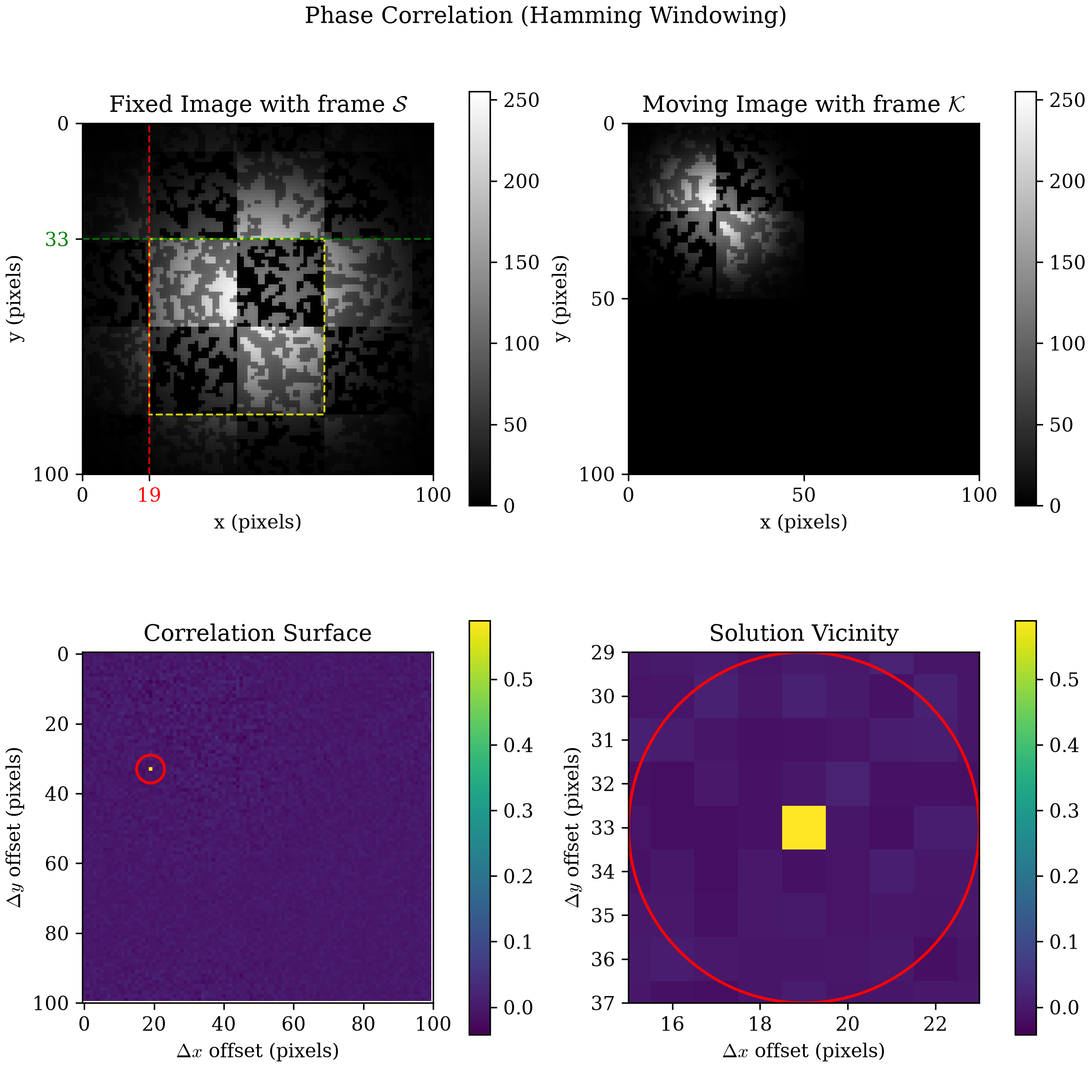
four-panel composite for phase correlation with Hamming windowing: fixed image and moving image both darken toward their own edges but not fully to black, same correlation surface peak location as no windowing — Same shape and peak as No Windowing and Hann Windowing above too, and the same tapered Fixed Image/Moving Image panels — but Hamming's taper stops short of exactly 0 at the edges (around $0.08$ , per Windowing), trading a little residual discontinuity for a narrower main lobe, visible here as a fainter, not-quite-black edge compared to Hann's above. See Peak Prominence below for how that plays out numerically against Hann.

Peak Prominence

That sharpness isn't just a visual impression. Define a correlation surface's peak prominence $P$ as how many standard deviations above its own mean the peak sits — a scale-independent way to compare surfaces with very different raw units (CC's arbitrary sums, NCC/ZNCC's $[- 1, 1]$ -bounded values, phase correlation's own normalized range):

$P (C) := \frac{max ( C ) - C ˉ}{σ _{C}}, \overset{ˉ}{C} := \frac{1}{n} i = 1 \sum n C_{i}, σ_{C} := \frac{1}{n} i = 1 \sum n (C_{i} - \overset{ˉ}{C})^{2}$

for a correlation surface $C$ flattened to its $n$ values. By this measure, all three phase correlation surfaces above are dramatically higher than any spatial-domain criterion — and windowing raises that further still, even on this book's clean, noise-free synthetic images:

CC: prominence P = 4.93
NCC: prominence P = 5.60
ZCC: prominence P = 5.48
ZNCC: prominence P = 5.60
Phase correlation (no windowing): prominence P = 38.91
Phase correlation (Hann): prominence P = 56.76
Phase correlation (Hamming): prominence P = 58.95

A histogram of each surface's own values makes the same result visual: each panel's dashed red line is that surface's peak, at the value computed above.

import matplotlib.pyplot as plt
from dictk.correlation import cc, ncc, zcc, zncc, phase_correlation, WindowingMethod

surfaces = {
    "CC": cc(kernel=kernel, search=search),
    "NCC": ncc(kernel=kernel, search=search),
    "ZCC": zcc(kernel=kernel, search=search),
    "ZNCC": zncc(kernel=kernel, search=search),
    "Phase correlation\n(no windowing)": phase_correlation(kernel=kernel, search=search),
    "Phase correlation\n(Hann)": phase_correlation(kernel=kernel, search=search, windowing=WindowingMethod.HANN),
    "Phase correlation\n(Hamming)": phase_correlation(kernel=kernel, search=search, windowing=WindowingMethod.HAMMING),
}

plt.rcParams.update({"font.family": "serif", "mathtext.fontset": "cm"})
fig, axes = plt.subplots(4, 2, figsize=(11, 16), constrained_layout=True)
for ax, (name, surface) in zip(axes.flat, surfaces.items()):
    flat = surface.ravel()
    prominence = (flat.max() - flat.mean()) / flat.std()
    ax.hist(flat, bins=60, color="black", alpha=0.7)
    ax.axvline(flat.max(), color="red", linestyle="--", linewidth=1.5)
    ax.set_yscale("log")
    ax.set_title(f"{name}: $P = {prominence:.1f}$")
    ax.set_xlabel("surface value")
    ax.set_ylabel("frequency")
axes.flat[-1].axis("off")  # 7 panels in a 4x2 grid -- last slot stays empty
fig.savefig("correlation_visualization_prominence.png", dpi=300)

Saved: correlation_visualization_prominence.png

seven histogram panels, one per correlation criterion/windowing combination, each showing the distribution of that surface's own values with a dashed red line marking its peak; the four spatial criteria show a broad bell-like spread with the peak in a modestly separated upper tail, while the three phase correlation panels each show a narrow spike near zero with its peak isolated far to the right, well beyond any other bar, windowed variants more so — Each surface's own value distribution (log-scaled frequency, 60 bins), dashed red line at its peak — every dashed line marks the same $r_{S K / S} = (19, 33)$ -pixel location `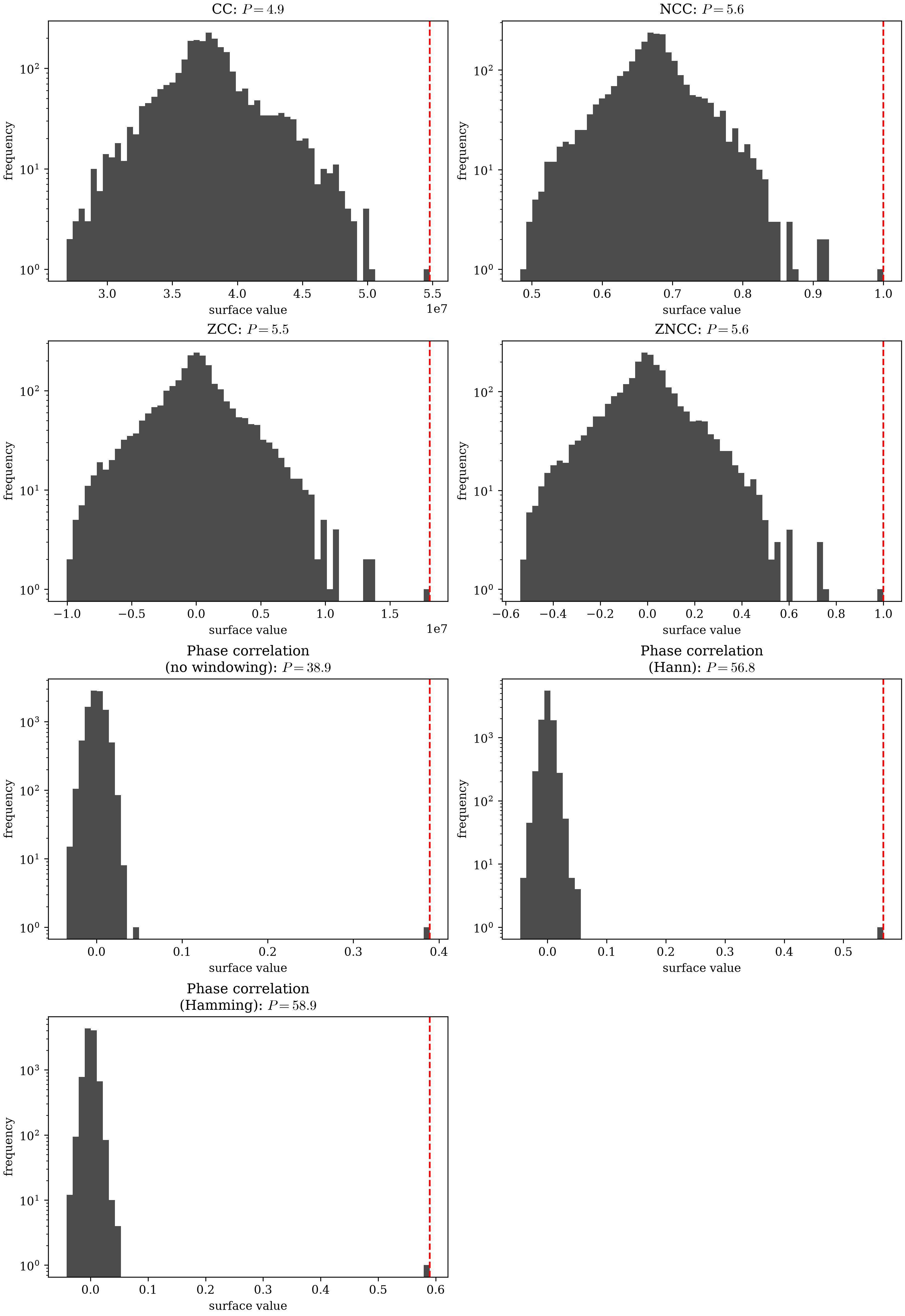locate` already found in Cross Correlation (CC), just plotted by value here rather than position. CC/NCC/ZCC/ZNCC's peaks sit a short, visible distance beyond their own bulk. All three phase correlation panels sit in a class of their own — an empty gap separates each peak from every other value its surface takes on — and windowing (Hann, Hamming) narrows that surface's own bulk further still, widening the gap even more.

Windowing's effect here isn't about relocating the peak — all seven surfaces, spatial and Fourier alike, land on the same $r_{S K / S} = (19, 33)$ -pixel offset — it's about how far above the rest of the surface that peak stands. No-windowing phase correlation already beats every spatial criterion by a wide margin (prominence 38.91 vs. ZNCC's 5.60, the best of the four); Hann windowing raises that to 56.76 and Hamming to 58.95, by lowering the energy the leaking, untapered edges were contributing everywhere else on the surface, so the same peak stands out further above that now-lower background. Hann and Hamming land close to each other, both clearly above no windowing — a real, measurable benefit even before considering the noisier, less-clean real-world images this book's synthetic ones deliberately simplify away.

Phase correlation's peak already stands roughly seven times taller above its own background, relative to the surface's own spread, than even ZNCC — the most robust of the four spatial criteria — before windowing is even applied. That sharpness, not just brightness/contrast invariance, is a second, independent reason dictk.translation.locate is built on phase correlation rather than a spatial-domain criterion: a sharper peak is easier to locate with confidence and precision, and harder to confuse with a nearby runner-up. locate accepts the same windowing parameter too (see Windowing) — the prominence gain above isn't unique to the surface phase_correlation() exposes for visualization; it applies wherever the same FFT-based comparison runs, locate included.

Keyboard shortcuts

dictk User Guide