Finite Element Method

A finite element mesh is a collection of nodes (points) connected into elements — small regions used to interpolate a quantity of interest (e.g. displacement) across the whole domain. Multi-Point Motion (covered later in this book) builds exactly this kind of nodal point collection and, in Tracking the Grid, tracks every one of its 12 points to its current position — exactly the per-node displacement data a mesh needs to represent how an object deformed.

Kernel Size First also covers the kernel-size-versus-point-spacing tradeoff involved in getting that per-node data reliably — the same considerations apply whether the points come from a toy grid or a real mesh.

Once every node's current position is known, an actual finite element mesh still needs one more thing this page doesn't provide: element connectivity — which nodes join together into which elements. Building that connectivity is future work, not implemented here; what this page covers below is the element formulation that connectivity would plug into — shape functions, strain, and deformation gradient, for the four-node quadrilateral element.

Four-Noded Quadrilateral Finite Element (Q4)

The four-node quadrilateral element is one of the most commonly used elements in 2D FEA. It has four corner nodes, with each node having two degrees of freedom (DOFs): displacements in the $X$ and $Y$ directions.

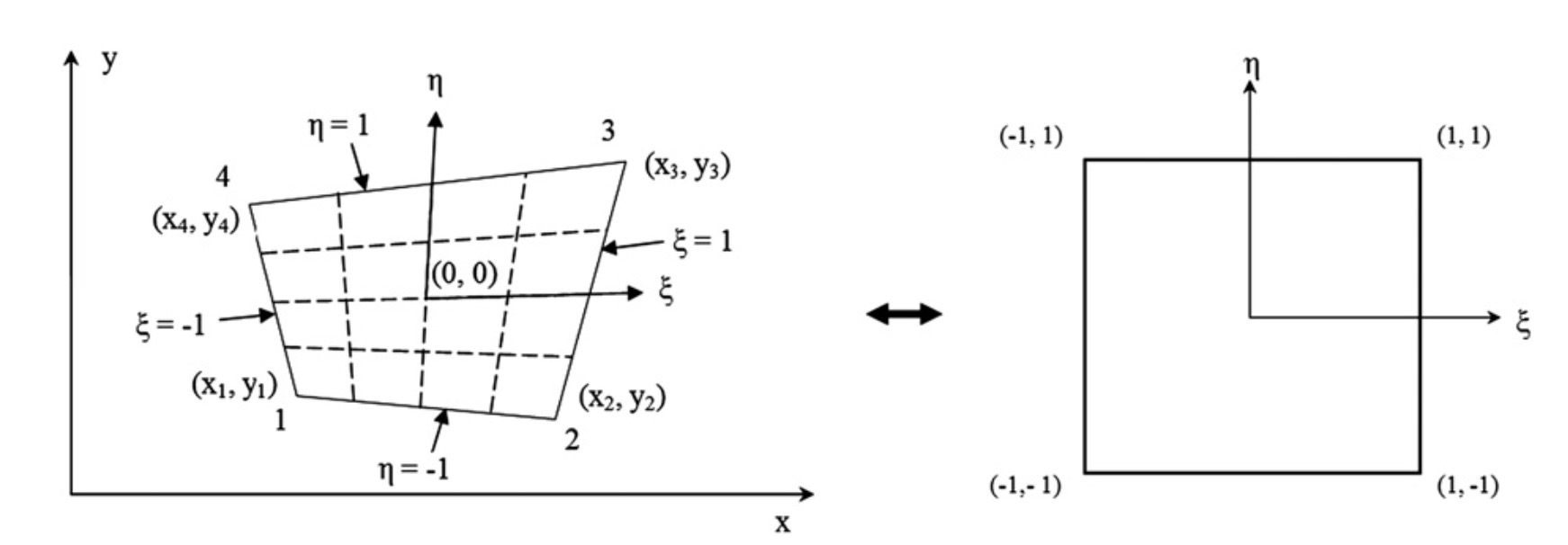
Image credit: James et al.¹

Note: Since we are using a finite deformation continuum mechanics framework, we will use $X$ and $Y$ (instead of $x$ and $y$ in the James et al. figure above).

Shape Functions

For the element in local coordinates $(\xi ,\eta )\in [-1,1]\times [-1,1]$, the bilinear shape functions are defined:

$$\begin{array}{rl}{N}_1(\xi ,\eta )& :=\frac{1}{4}(1-\xi )(1-\eta )\\ N_2(\xi ,\eta )& :=\frac{1}{4}(1+\xi )(1-\eta )\\ N_3(\xi ,\eta )& :=\frac{1}{4}(1+\xi )(1+\eta )\\ N_4(\xi ,\eta )& :=\frac{1}{4}(1-\xi )(1+\eta )\end{array}$$

The shape functions satisfy the following properties:

• Kronecker delta property: $N_a({\xi }_b,{\eta }_b)={\delta }_{ab}$ (equals 1 at node $a$, 0 at other nodes)
• Partition of unity: ${\sum }_{a=1}^4{N}_a(\xi ,\eta )=1$ for all $(\xi ,\eta )$

Local Coordinates

The key concept in finite element analysis is the isoparametric mapping between the local coordinate system and the global coordinate system.

This mapping allows:

• Integration to be performed on the local domain (parent element)
• Handling of arbitrarily shaped quadrilaterals
• Use of the same shape functions for geometry and displacement (isoparametric concept)

The isoparametric coordinates $(\xi ,\eta )$ range from $-1$ to $+1$ in both the $X$ and $Y$ directions.

The mapping between global coordinates $(X,Y)$ and local coordinates is introduced as a linear combination of local shape functions $N_{\mathrm{node}}(\mathbf{X})$:

$$\mathbf{X}(\mathbf{\xi })=\left\{\begin{array}{c}X(\xi ,\eta )\\ Y(\xi ,\eta )\end{array}\right\}=\sum _{a=1}^4{N}_a(\mathbf{\xi }){\mathbf{X}}_a=\sum _{a=1}^4{N}_a(\xi ,\eta )\left\{\begin{array}{c}{X}_a\\ Y_a\end{array}\right\}$$

where $(X_a,Y_a)$ is the position of node $a$, and $a=1\dots 4$.

Shape Function Derivatives in Local Coordinates

The derivatives with respect to the local coordinate system are

$$\frac{\partial N_a(\xi ,\eta )}{\partial \xi }=\frac{1}{4}\left[\begin{array}{c}-(1-\eta )\\ (1-\eta )\\ (1+\eta )\\ -(1+\eta )\end{array}\right],\frac{\partial N_a(\xi ,\eta )}{\partial \eta }=\frac{1}{4}\left[\begin{array}{c}-(1-\xi )\\ -(1+\xi )\\ (1+\xi )\\ (1-\xi )\end{array}\right]$$

These are assembled into a $2\times 4$ matrix:

$$\frac{\partial \mathbf{N}(\mathbf{\xi })}{\partial \mathbf{\xi }}={\left[\begin{array}{cccc}\frac{\partial N_1}{\partial \xi }& \frac{\partial N_2}{\partial \xi }& \frac{\partial N_3}{\partial \xi }& \frac{\partial N_4}{\partial \xi }\\ \frac{\partial N_1}{\partial \eta }& \frac{\partial N_2}{\partial \eta }& \frac{\partial N_3}{\partial \eta }& \frac{\partial N_4}{\partial \eta }\end{array}\right]}_{2\times 4}$$

Jacobian Matrix

The Jacobian matrix ${\mathbf{j}}_0$ relates derivatives in local coordinates to derivatives in global coordinates. It is important to include the "matrix" part of "Jacobian matrix". It is distinct from the Jacobian of the Deformation Gradient $J$, which is a scalar value (not a matrix). For nodal coordinates organized as:

$$\mathbf{X}={\left[\begin{array}{cc}{X}_1& Y_1\\ X_2& Y_2\\ X_3& Y_3\\ X_4& Y_4\end{array}\right]}_{4\times 2}$$

the Jacobian matrix ${\mathbf{j}}_0$ is computed as:

$${\mathbf{j}}_0(\mathbf{\xi }):=\frac{\partial \mathbf{X}(\mathbf{\xi })}{\partial \mathbf{\xi }}={\left[\begin{array}{cc}\frac{\partial X}{\partial \xi }& \frac{\partial Y}{\partial \xi }\\ \frac{\partial X}{\partial \eta }& \frac{\partial Y}{\partial \eta }\end{array}\right]}_{2\times 2}=\frac{\partial \mathbf{N}(\mathbf{\xi })}{\partial \mathbf{\xi }}\cdot \mathbf{X}$$

The individual components (dropping the ${\bullet }_0$ reference configuration notation to avoid subscript confusion) are:

$$\begin{array}{rl}{j}_{11}& =\frac{\partial X}{\partial \xi }=\sum _{a=1}^4\frac{\partial N_a}{\partial \xi }{X}_a\\ j_{12}& =\frac{\partial Y}{\partial \xi }=\sum _{a=1}^4\frac{\partial N_a}{\partial \xi }{Y}_a\\ j_{21}& =\frac{\partial X}{\partial \eta }=\sum _{a=1}^4\frac{\partial N_a}{\partial \eta }{X}_a\\ j_{22}& =\frac{\partial Y}{\partial \eta }=\sum _{a=1}^4\frac{\partial N_a}{\partial \eta }{Y}_a\end{array}$$

Shape Function Derivatives in Global Coordinates

The transformation from local to global coordinate derivatives requires the inverse Jacobian matrix through the chain rule. Since

$$\frac{\partial N_a}{\partial X}=\frac{\partial N_a}{\partial \xi }\frac{\partial \xi }{\partial X}+\frac{\partial N_a}{\partial \eta }\frac{\partial \eta }{\partial X}$$

$$\frac{\partial N_a}{\partial Y}=\frac{\partial N_a}{\partial \xi }\frac{\partial \xi }{\partial Y}+\frac{\partial N_a}{\partial \eta }\frac{\partial \eta }{\partial Y}$$

then

$$\left[\begin{array}{c}\frac{\partial N_a}{\partial X}\\ \frac{\partial N_a}{\partial Y}\end{array}\right]={\left[\begin{array}{cc}\frac{\partial \xi }{\partial X}& \frac{\partial \eta }{\partial X}\\ \frac{\partial \xi }{\partial Y}& \frac{\partial \eta }{\partial Y}\end{array}\right]}_{2\times 2}\left[\begin{array}{c}\frac{\partial N_a}{\partial \xi }\\ \frac{\partial N_a}{\partial \eta }\end{array}\right]={\mathbf{j}}_0^{-1}(\mathbf{X})\left[\begin{array}{c}\frac{\partial N_a}{\partial \xi }\\ \frac{\partial N_a}{\partial \eta }\end{array}\right]$$

In matrix form for all shape functions:

$$\frac{\partial \mathbf{N}}{\partial \mathbf{X}}={\mathbf{j}}_0^{-1}\cdot \frac{\partial \mathbf{N}}{\partial \mathbf{\xi }}$$

where:

$$\frac{\partial \mathbf{N}}{\partial \mathbf{X}}={\left[\begin{array}{cccc}\frac{\partial N_1}{\partial X}& \frac{\partial N_2}{\partial X}& \frac{\partial N_3}{\partial X}& \frac{\partial N_4}{\partial X}\\ \frac{\partial N_1}{\partial Y}& \frac{\partial N_2}{\partial Y}& \frac{\partial N_3}{\partial Y}& \frac{\partial N_4}{\partial Y}\end{array}\right]}_{2\times 4}$$

Displacement Field

The displacement $\mathbf{u}(\mathbf{X})$ is defined as the difference between the current configuration $\mathbf{\phi }(\mathbf{X})$ and the reference configuration $\mathbf{X}$,

$$\mathbf{u}(\mathbf{X}):=\mathbf{\phi }(\mathbf{X})-\mathbf{X}$$

The displacement field within the element is interpolated using shape functions:

$$\mathbf{u}(\xi ,\eta )=\left\{\begin{array}{c}u(\xi ,\eta )\\ v(\xi ,\eta )\end{array}\right\}=\sum _{a=1}^4{N}_a(\mathbf{\xi }){\mathbf{u}}_a=\sum _{a=1}^4{N}_a(\xi ,\eta )\left\{\begin{array}{c}{u}_a\\ v_a\end{array}\right\}$$

where $(u_a,v_a)$ is the respective $(X,Y)$ displacement of node $a$, and $a=1\dots 4$.

Displacement Gradient

$${\nabla }_0\mathbf{u}(\mathbf{X})={\left[\begin{array}{cc}\frac{\partial u}{\partial X}& \frac{\partial u}{\partial Y}\\ \frac{\partial v}{\partial X}& \frac{\partial v}{\partial Y}\end{array}\right]}_{2\times 2}$$

Each component is computed using the chain rule:

$$\begin{array}{rl}\frac{\partial u}{\partial X}& =\sum _{a=1}^4\frac{\partial N_a}{\partial X}{u}_a\\ \frac{\partial u}{\partial Y}& =\sum _{a=1}^4\frac{\partial N_a}{\partial Y}{u}_a\\ \frac{\partial v}{\partial X}& =\sum _{a=1}^4\frac{\partial N_a}{\partial X}{v}_a\\ \frac{\partial v}{\partial Y}& =\sum _{a=1}^4\frac{\partial N_a}{\partial Y}{v}_a\end{array}$$

In compact matrix notation:

$${\nabla }_0\mathbf{u}={\left(\frac{\partial \mathbf{N}}{\partial \mathbf{X}}\cdot \mathbf{u}\right)}^T$$

where $\mathbf{u}$ is the nodal displacement matrix:

$$\mathbf{u}={\left[\begin{array}{cc}{u}_1& v_1\\ u_2& v_2\\ u_3& v_3\\ u_4& v_4\end{array}\right]}_{4\times 2}$$

See Displacement Gradient for more information.

Deformation Gradient

The deformation gradient tensor $\mathbf{F}(\mathbf{X})$ maps material points in the reference configuration $\mathbf{X}$ to their positions in the current (deformed) configuration $\mathbf{\phi }$:

$$\mathbf{F}(\mathbf{X}):=\frac{\partial \mathbf{\phi }(\mathbf{X})}{\partial \mathbf{X}}$$

Because $\mathbf{u}(\mathbf{X})=\mathbf{\phi }(\mathbf{X})-\mathbf{X}$,

$${\nabla }_0\mathbf{u}=\mathbf{F}-\mathbf{I}⟹\mathbf{F}={\nabla }_0\mathbf{u}+\mathbf{I}$$

Explicitly:

$$\mathbf{F}=\left[\begin{array}{cc}{F}_{11}& F_{12}\\ F_{21}& F_{22}\end{array}\right]=\left[\begin{array}{cc}\frac{\partial u}{\partial X}+1& \frac{\partial u}{\partial Y}\\ \frac{\partial v}{\partial X}& \frac{\partial v}{\partial Y}+1\end{array}\right]$$

The determinant $J:=\det (\mathbf{F})$ represents the local volume ratio and must be positive for physically admissible deformations. See Deformation Gradient and Jacobian of the Deformation Gradient for more information.

Gauss Points

To evaluate quantities that depend on the displacement field and its gradient, such as strain, we use Gaussian Quadrature. We don't typically calculate quantities at the nodes. Rather, we quantify strain at specific integration points (also known as Gauss points) where mathematical precision is the highest.

For a 2D quadrilateral element, we typically use a $2\times 2$ Gauss rule. The integration points are located in the local coordinate system $(\xi ,\eta )$ at

$$\xi ,\eta \in \left\{\pm \frac{1}{\sqrt{3}}\right\}\approx \pm 0.57735$$

References

1. James KA, Lee E, Martins JR. Stress-based topology optimization using an isoparametric level set method. Finite Elements in Analysis and Design. 2012 Oct 1;58:20-30. link ↩