Multi-Point Motion
Single Point Motion tracked exactly one point, , between a reference and current image. Digital image correlation was illustrated in the context of that single point. Now, we turn to consider many points at once. A collection of tracked points will serve as the nodes of a finite element mesh. This page shows how to track many points simultaneously, and motivates the connection to the Finite Element Method (FEM).
Commercial DIC Context
Commercial DIC software sets up a measurement in a specific order, and
it runs opposite to order presented on this page.
The reversal is a deliberate choice because we have not yet introduced
subpixel accuracy. After subpixel accuracy is
discussed, dictk will follow the same order used by commerical DIC software,
described next:
Kernel size comes first. A kernel must contain enough distinctive texture to correlate reliably. An image will contain features (e.g., a speckle pattern feature such as a corner or edge). The goal is to get enough (but not too many) pixels to describe a feature. Too few pixels cause the kernel contents to be ambiguous. Too many pixels cause the kernel to be saturated with pixels that do not participate in the feature, resulting in poor-to-no correlation. Too many pixels also can also increase computational cost beyond what is necessary for a successful correlation.
Ultimately, the size of the kernel is based on the speckle pattern's own feature size and the camera's resolution, which dictates the number of pixels per unit length present in the image.
Point spacing comes second. Once kernel size is fixed, point spacing (where to place each kernel center) follows from it.
- Some practitioners deliberately overlap neighboring kernels: A common convention is 50-75% overlap. So spacing works out to roughly a quarter to a half of the kernel's own side length — to oversample the field for a smoother reconstruction.
- Others keep kernels non-overlapping, so each point's own measurement stays independent of its neighbors': No two points ever look at the same underlying pixels.
Either way, the same tradeoff governs the choice: Too close, and neighboring kernels duplicate each other's content; too far apart, and the measurement undersamples the field.
The point grid becomes FEA nodes afterward, not before. Once tracking finishes, the resulting grid of measured points is what gets used as finite-element nodes. The mapping between DIC points and mesh points can be direct or indirect. Direct build a mesh directly from the DIC point cloud. Indirect uses the point cloud as an interpolation basis for a separately designed mesh. The FE mesh's density inherits the kernel-and-spacing choice for the correlation.
Let's continue with this example with a rather large choice for a pixel
size. Let kernel_margin_width=20 pixel and kernel_margin_height=20 pixel.
The kernel's side length is twice its margin: pixels.
This kernel is enough to contain plenty of distinctive texture
on astronaut0's uniformly-speckled, synthetic surface,
where no single location demands special care over another.
Heuristically, we typically use kernel sizes of 25 x 25 pixel, up to
35 x 35 pixel (considerably smaller than the 40 x 40 pixel used in this
example).
A common rule of thumb (no hard requirement behind it) is to keep a
kernel's own side length comfortably inside the point spacing —
the geometric floor for zero overlap is exact: with an isotropic
kernel (kernel_margin_width=kernel_margin_height), two neighboring
kernels start overlapping once the kernel's own full side length
exceeds the spacing between their center points. For this example,
spacing has to reach
at least 40 pixels in both directions to clear that floor; right at
exactly 40 pixels, neighboring kernels would touch with zero gap
between them.
For now, we choose a point spacing not based on kernel size, but on locations that, given a prescribed stretch factor, will land exactly on an integer location in the deformed configuration. We need integer positions for now because we have not yet introduced subpixel accuracy.
Let spacing_x=50 px, spacing_y=55 px be the point spacing for
this page's example, keeping kernels non-overlapping (the second
convention named above) — both comfortably above that 40-pixel floor:
a 10-pixel gap in and a 15-pixel gap in , so every kernel's own
boundary will read as visibly separate from its neighbors', not merely
non-overlapping.
The following figure illustrates point spacing in the context the kernel's size:
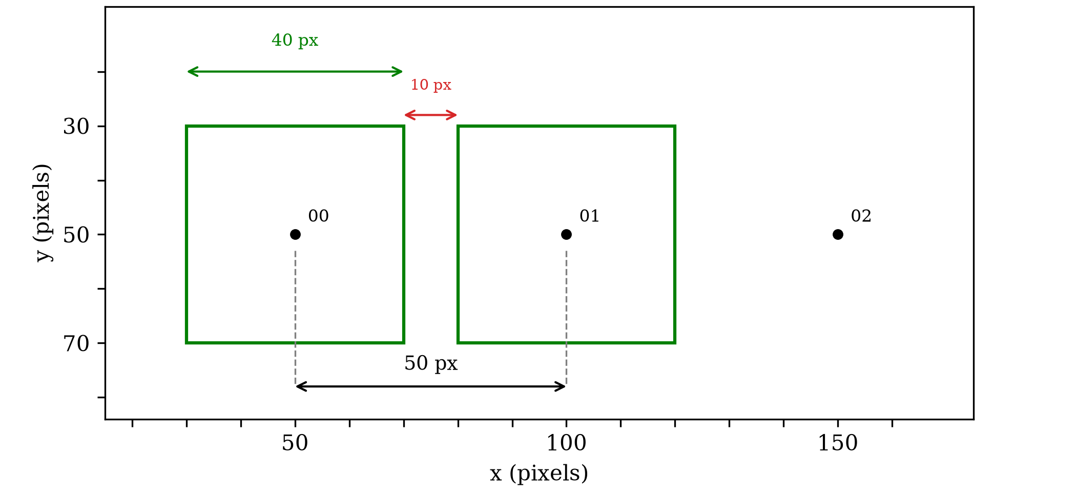
Show the figure-generating code
import matplotlib.pyplot as plt
import matplotlib.patches as patches
from dictk.image import PixelCoordinate

p0, p1, p2 = PixelCoordinate(x=50, y=50), PixelCoordinate(x=100, y=50), PixelCoordinate(x=150, y=50)
kernel_margin = 20

plt.rcParams.update({"font.family": "serif", "mathtext.fontset": "cm"})
fig, ax = plt.subplots(figsize=(7, 3.2), constrained_layout=True)

for p, label in [(p0, "00"), (p1, "01"), (p2, "02")]:
    ax.plot(p.x, p.y, "o", color="black", markersize=4)
    ax.annotate(label, (p.x, p.y), textcoords="offset points", xytext=(6, 6), fontsize=8)

for p in (p0, p1):
    ax.add_patch(patches.Rectangle(
        (p.x - kernel_margin, p.y - kernel_margin),
        2 * kernel_margin, 2 * kernel_margin,
        edgecolor="green", facecolor="none", linewidth=1.5,
    ))

box_top = p0.y - kernel_margin      # 30
box_bottom = p0.y + kernel_margin   # 70

# 50-pixel point spacing. The dashed guide lines start near each point
# (nearly touching its marker) and run down through its kernel box to
# the dimension line just below the boxes. Arrow flush with the dashed
# lines (shrinkA/shrinkB=0); label centered at the true midpoint between
# the box bottom and the dimension line.
dim_y = box_bottom + 8
for p in (p0, p1):
    ax.plot([p.x, p.x], [p.y + 3, dim_y], color="gray", linestyle="--", linewidth=0.8)
ax.annotate("", xy=(p0.x, dim_y), xytext=(p1.x, dim_y), arrowprops=dict(arrowstyle="<->", color="black", shrinkA=0, shrinkB=0))
ax.text((p0.x + p1.x) / 2, (box_bottom + dim_y) / 2, "50 px", ha="center", va="center", fontsize=9)

# 40-pixel kernel width, flush with the box's own left/right edges
# (shrinkA/shrinkB=0 so the arrow isn't inset from those edges).
top_y = box_top - 10
ax.annotate("", xy=(p0.x - kernel_margin, top_y), xytext=(p0.x + kernel_margin, top_y), arrowprops=dict(arrowstyle="<->", color="green", shrinkA=0, shrinkB=0))
ax.text(p0.x, top_y - 4, "40 px", ha="center", va="bottom", fontsize=8, color="green")

# 10-pixel gap between the two kernels' facing edges, moved up to the
# boxes' shared top edge, flush with the box's own edges (shrinkA/
# shrinkB=0), with the label on top of the dimension line.
gap_y = box_top - 2
ax.annotate("", xy=(p0.x + kernel_margin, gap_y), xytext=(p1.x - kernel_margin, gap_y), arrowprops=dict(arrowstyle="<->", color="tab:red", shrinkA=0, shrinkB=0))
ax.text(p0.x + kernel_margin + (p1.x - kernel_margin - (p0.x + kernel_margin)) / 2, gap_y - 4, "10 px", ha="center", va="bottom", fontsize=7, color="tab:red")

ax.set_xlim(15, 175)
ax.set_ylim(84, 8)

# Tick marks: 50/100/150 in x (the point positions), 40 pixels apart
# starting at 20; every 10 pixels in y, but text labels only at
# 30/50/70 (the box's top edge, the point row, and the box's bottom
# edge) -- a tight range with no dead space below the boxes, since the
# dimension line sits just beneath them.
xticks = list(range(20, 161, 10))
ax.set_xticks(xticks)
ax.set_xticklabels([str(v) if v in (50, 100, 150) else "" for v in xticks])
yticks = list(range(20, 81, 10))
ax.set_yticks(yticks)
ax.set_yticklabels([str(v) if v in (30, 50, 70) else "" for v in yticks])

ax.set_xlabel("x (pixels)")
ax.set_ylabel("y (pixels)")
ax.set_aspect("equal")
fig.savefig("multi_point_motion_spacing.png", dpi=300)
Saved: multi_point_motion_spacing.png
With kernel size and the point spacing it implies both settled, the point grid can be generated next.
Point Grid
A grid is an ordered, sequential collection of points, arranged in a rectilinear
pattern.
The function dictk.grid.generate creates
a grid that spans some number of points along and along ,
with some spacing between adjacent points along each axis.
The count of points along and along need not be equal, and the
spacing along and along need not be equal either. The grid is a
general rectangular collection of points, not necessarily a square or
uniformly-spaced one. spacing_x and spacing_y are in pixels.
This page uses astronaut0, the speckle pattern combined with the
astronaut photograph introduced in Image
Generation.
from dictk.image import read, PixelCoordinate
from dictk.plot import point_grid_plot
from dictk.grid import generate

reference_image = read(path="astronaut0.png")

points = generate(
    origin=PixelCoordinate(x=50, y=50),
    count_x=3,
    count_y=4,
    spacing_x=50,
    spacing_y=55,
)
point_grid_plot(
    image=reference_image,
    points=points,
    color="orange",
    figsize=(6.4, 4.8),
    path="multi_point_motion_grid.png",
)
Saved: multi_point_motion_grid.png
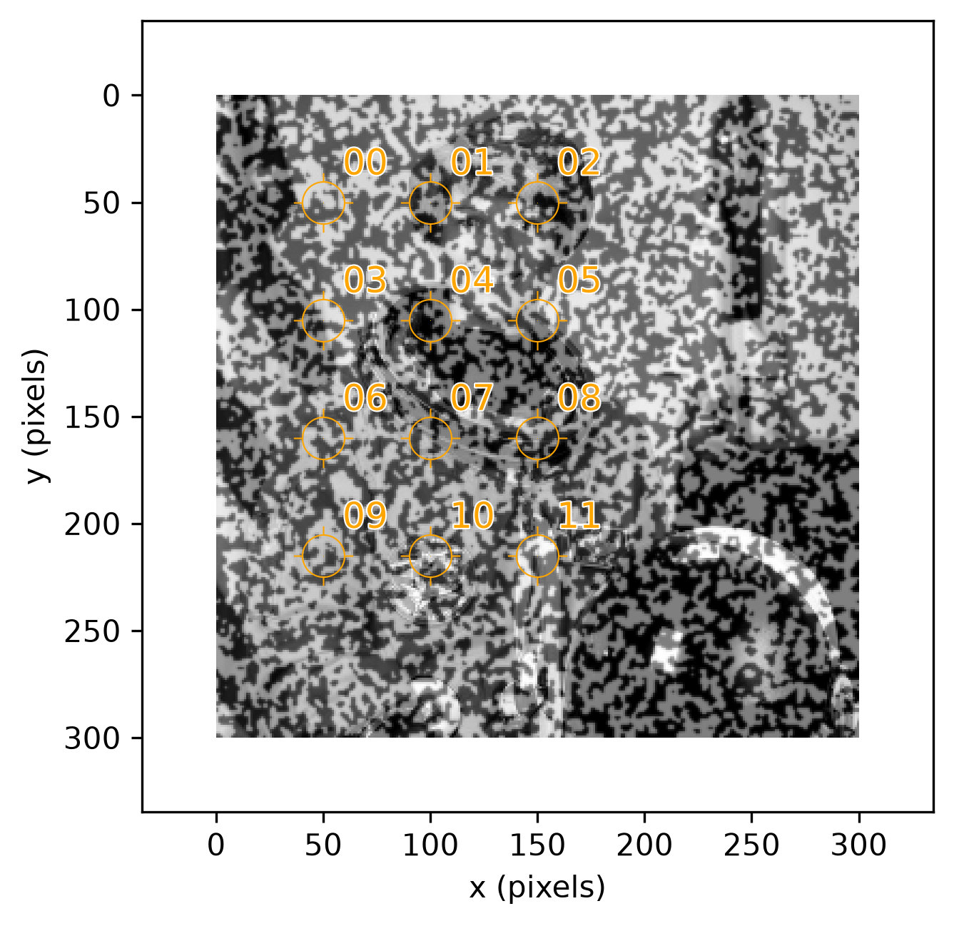
astronaut0 with a 3x4 grid of 12 points (count_x=3, count_y=4), spaced 50 pixels apart along and 55 pixels apart along (spacing_x=50, spacing_y=55), labeled 00-11 in row-major order (top-left to bottom-right).The reference coordinates in pixels for each point follow:
| Point | Reference Configuration | |
|---|---|---|
| (pixels) | (pixels) | |
| 00 | 50 | 50 |
| 01 | 100 | 50 |
| 02 | 150 | 50 |
| 03 | 50 | 105 |
| 04 | 100 | 105 |
| 05 | 150 | 105 |
| 06 | 50 | 160 |
| 07 | 100 | 160 |
| 08 | 150 | 160 |
| 09 | 50 | 215 |
| 10 | 100 | 215 |
| 11 | 150 | 215 |
from dictk.image import translate

dx, dy = -6, 8
current_image = translate(arr=reference_image, dx=dx, dy=dy)
Tracking the Grid
Every point's own kernel and search area, using the kernel size chosen
above, look like this.
dictk.plot.point_grid_boxes_plot
draws one box type per call, so kernel and search area each get their own
figure — each point's own box gets its own color and its own legend
entry (kernel 00, kernel 01, ..., kernel 11), cycling through a
12-color palette (using matplotlib's Tableau colormap):
from dictk.plot import point_grid_boxes_plot

point_grid_boxes_plot(
    image=reference_image,
    points=points,
    margin_width=20,
    margin_height=20,
    label_prefix="kernel",
    figsize=(6.4, 4.8),
    path="multi_point_motion_kernels.png",
)
Saved: multi_point_motion_kernels.png
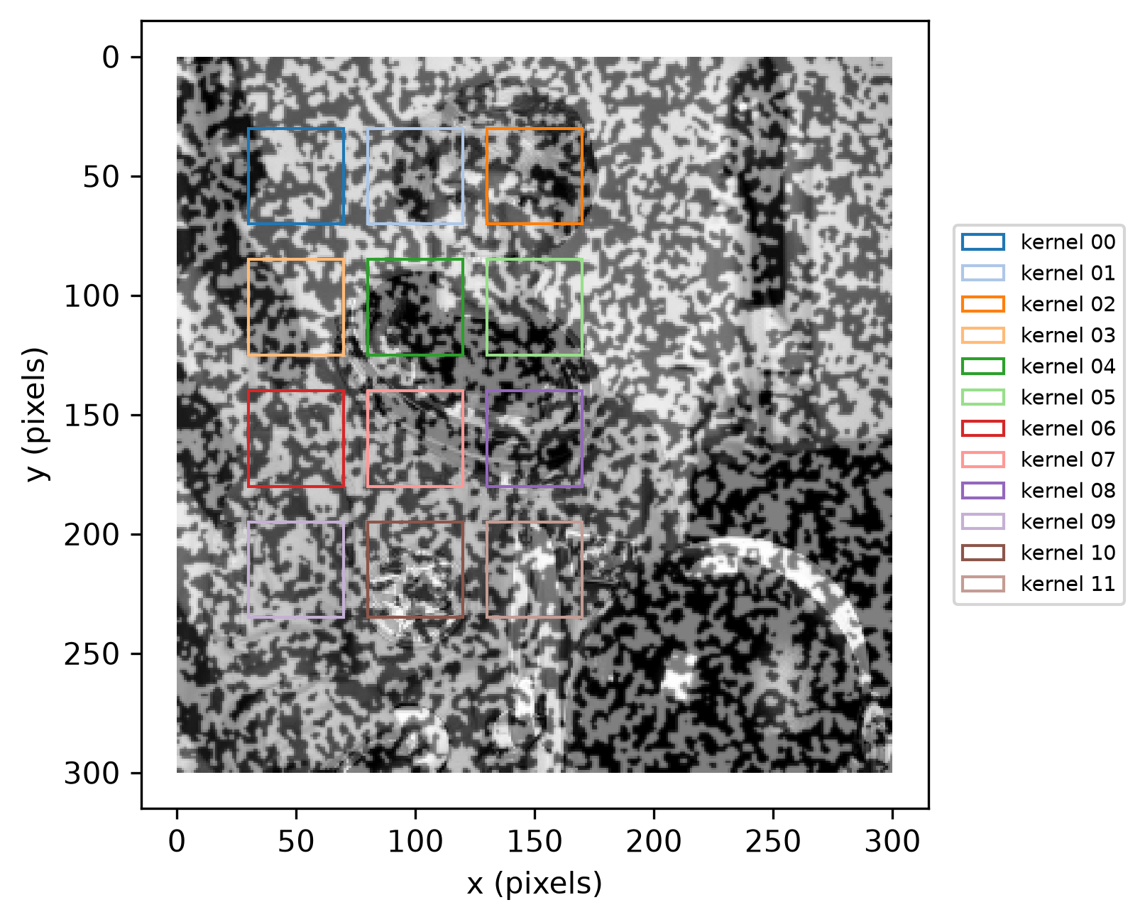
margin_width=20, margin_height=20).The kernel comes from reference_image. The search area comes from
current_image instead — still centered on each point's reference
position (search_centers defaults to reference_points), since the
point's true displacement is exactly what tracking is trying to find:
point_grid_boxes_plot(
    image=current_image,
    points=points,
    margin_width=48,
    margin_height=52,
    label_prefix="search area",
    figsize=(6.4, 4.8),
    path="multi_point_motion_search.png",
)
Saved: multi_point_motion_search.png
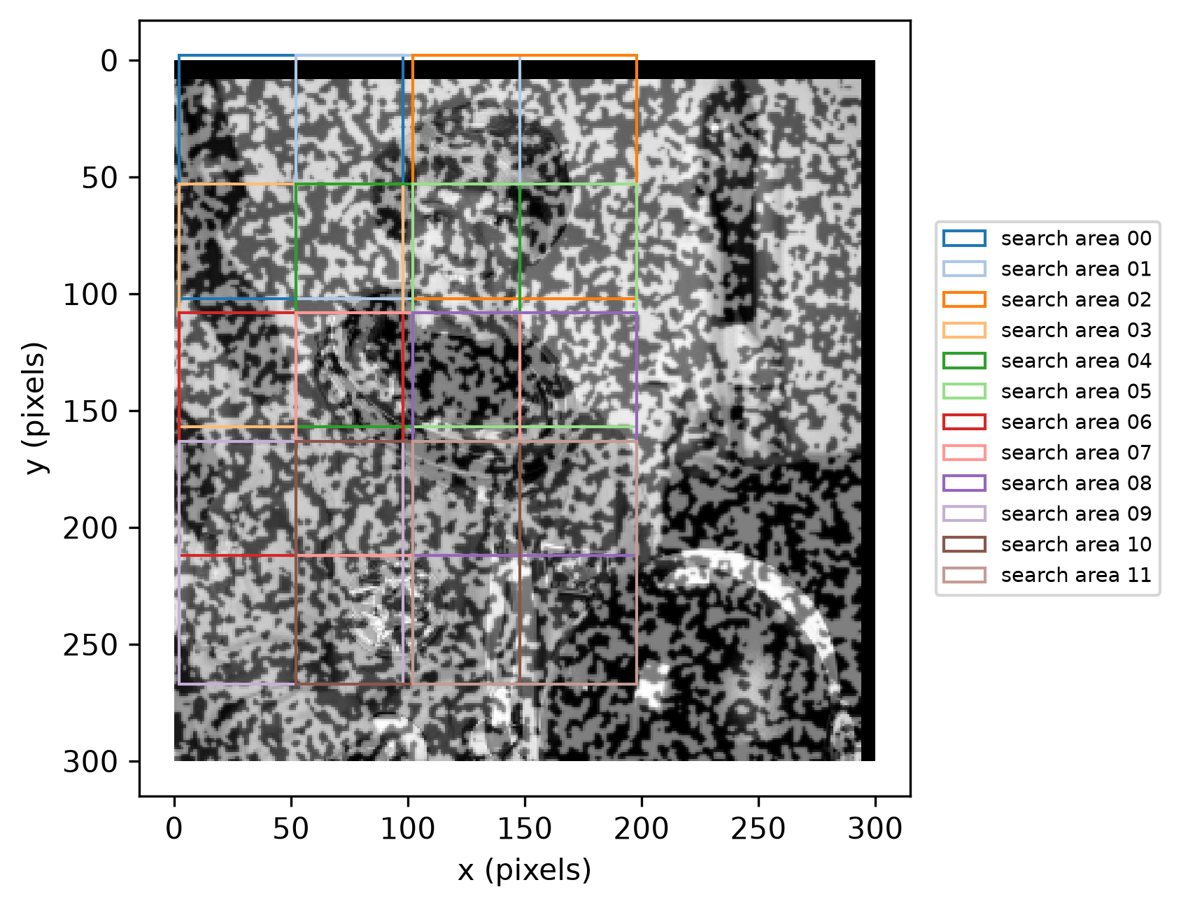
margin_width=48, margin_height=52), drawn on current_image — the region actually searched — and still centered on each point's reference position.Nothing requires the kernel to be isotropic — dictk supports an
independent margin per axis just as easily. The equal 20/20 above is
a deliberate choice to illustrate that dictk supports both isotropic and
non-isotropic margins, not a consequence of spacing_x and spacing_y
being unequal forcing one shape or the other.
The search area, by contrast, keeps a clearly
non-isotropic shape: search_margin_width=48, search_margin_height=52
— just under the point spacing itself, comfortably containing the known
-pixel displacement with plenty of room to spare, while staying
just shy of spacing_x/spacing_y rather than matching them outright.
That much slack still means search areas overlap their neighbors heavily
and run off the image at the edges, which is harmless:
subimage zero-pads whatever falls
outside current_image. Unlike kernels, search areas that overlap cost
nothing aside from redundant computation; there's no accuracy downside to
searching the same region for two different points.
One important practical detail: phase_cross_correlation
requires the kernel and search area to be exactly the same shape. So
dictk.translation.locate doesn't
crop the search area down to the kernel's size; rather, it zero-pads the kernel up to match the search area's size. Here a
40x40 kernel is zero-padded up to the search area's 96x104 size.
Note: In practice, kernel size has little effect on FFT runtime once a search area is chosen — the transform zero-pads the kernel up to match the search area's own size. Shrinking an already-small kernel further doesn't make the correlation any faster.
Single Point Motion
confirmed that a single point's found position matches a known
displacement exactly. Reuse current_image from Point
Grid — the same -pixel
displacement. The same idea, applied to all 12 points in the grid at
once, is exactly what a real DIC workflow looks like.
dictk.grid.locate tracks all 12 points
in one call. It doesn't do the correlation itself — it calls
dictk.translation.locate once
per point, and that function is dictk's actual FFT-based DIC engine: for
each point it extracts a kernel from reference_image and a search area
from current_image, then locates the kernel within the search area via
skimage.registration.phase_cross_correlation — FFT-based phase
cross-correlation, not a spatial-domain sliding-window search (see
Correlation Criteria for the
single-point version of this same technique).
Twelve points means twelve independent calls into that engine, using the
same kernel and search-area sizes visualized above:
from dictk.grid import locate

found = locate(
    reference_image=reference_image,
    current_image=current_image,
    reference_points=points,
    kernel_margin_width=20,
    kernel_margin_height=20,
    search_margin_width=48,
    search_margin_height=52,
)
Point  found        expected     match
00      44,58       44,58       True
01      94,58       94,58       True
02     144,58      144,58       True
03      44,113      44,113      True
04      94,113      94,113      True
05     144,113     144,113      True
06      44,168      44,168      True
07      94,168      94,168      True
08     144,168     144,168      True
09      44,223      44,223      True
10      94,223      94,223      True
11     144,223     144,223      True
Every one of the 12 found positions matches reference_points[i] + (dx, dy) exactly — not approximately, the same exact-integer-pixel guarantee
Single Point Motion established for one point,
now confirmed across the whole grid at once:
from dictk.plot import point_grid_plot

point_grid_plot(
    image=current_image,
    points=found,
    color="orange",
    figsize=(6.4, 4.8),
    path="multi_point_motion_found.png",
)
Saved: multi_point_motion_found.png
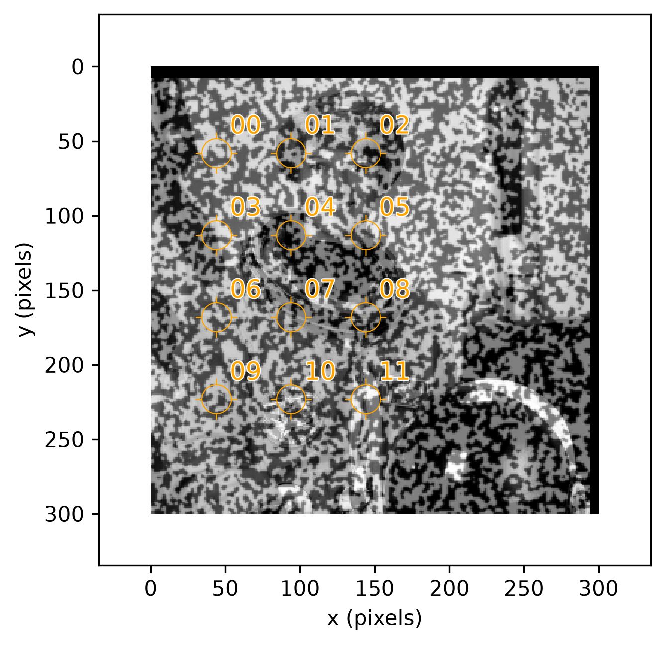
That every point was found exactly is expected, not a coincidence: the
kernel margins above were chosen to roughly follow the rule of thumb, not
to violate it. What the rule of thumb actually buys is robustness, not
correctness on an easy case like this one — a kernel needs enough
distinctive texture to locate reliably, and astronaut0 is a clean,
synthetic image with strong texture everywhere and no noise. A smaller,
more aggressively undersized kernel would likely still have worked here
too; it's on real, noisier imagery, or content with repetitive texture,
that a larger kernel's extra context resolves an ambiguity a smaller one
can't.
Data Download
Every image this page used is downloadable below, as a TIFF. Download files individually, or all at once: one compressed zip file bundles every full image (reference and current), every kernel, and every search area.
import zipfile
import imageio.v3 as iio

images = {"astronaut0.tiff": reference_image, "astronaut1.tiff": current_image}
for i, point in enumerate(points):
    origin = PixelCoordinate(x=point.x - kernel_margin, y=point.y - kernel_margin)
    images[f"kernel_{i:02d}.tiff"] = subimage(
        image=reference_image, origin=origin, width=2 * kernel_margin, height=2 * kernel_margin
    )
for i, point in enumerate(points):
    origin = PixelCoordinate(x=point.x - search_margin_width, y=point.y - search_margin_height)
    images[f"search_area_{i:02d}.tiff"] = subimage(
        image=current_image, origin=origin, width=2 * search_margin_width, height=2 * search_margin_height
    )

with zipfile.ZipFile("multi_point_motion_data.zip", "w", zipfile.ZIP_DEFLATED) as zf:
    for name, arr in images.items():
        zf.writestr(name, iio.imwrite("<bytes>", arr, extension=".tiff"))
Download all: multi_point_motion_data.zip (26 files, 291 KB)
Full Images
astronaut0.tiffisreference_image.astronaut1.tiffiscurrent_image—reference_imagedisplaced down and to the left by pixels, the same displacement Tracking the Grid tracked:
from dictk.image import write

write(arr=reference_image, path="astronaut0.tiff")
write(arr=current_image, path="astronaut1.tiff")
| File | Description |
|---|---|
| astronaut0.tiff | Reference image, 300x300 pixels |
| astronaut1.tiff | Current image, displaced by (dx, dy) = (-6, 8) pixels |
Kernels
Every point's kernel, extracted from reference_image — the same 12
boxes shown in Tracking the Grid (kernel_margin_width=20,
kernel_margin_height=20, 40x40 pixels each):
from dictk.image import subimage, write

kernel_margin = 20
for i, point in enumerate(points):
    origin = PixelCoordinate(x=point.x - kernel_margin, y=point.y - kernel_margin)
    kernel = subimage(image=reference_image, origin=origin, width=2 * kernel_margin, height=2 * kernel_margin)
    write(arr=kernel, path=f"kernel_{i:02d}.tiff")
| File | Point | Origin (pixels) |
|---|---|---|
| kernel_00.tiff | 00 | (30, 30) |
| kernel_01.tiff | 01 | (80, 30) |
| kernel_02.tiff | 02 | (130, 30) |
| kernel_03.tiff | 03 | (30, 85) |
| kernel_04.tiff | 04 | (80, 85) |
| kernel_05.tiff | 05 | (130, 85) |
| kernel_06.tiff | 06 | (30, 140) |
| kernel_07.tiff | 07 | (80, 140) |
| kernel_08.tiff | 08 | (130, 140) |
| kernel_09.tiff | 09 | (30, 195) |
| kernel_10.tiff | 10 | (80, 195) |
| kernel_11.tiff | 11 | (130, 195) |
Search Areas
Every point's search area, extracted from current_image — not
reference_image, since a search area is always a region of the current
image (see Tracking the Grid). The same 12 boxes shown there
(search_margin_width=48, search_margin_height=52, 96x104 pixels
each), still centered on each point's reference position:
search_margin_width, search_margin_height = 48, 52
for i, point in enumerate(points):
    origin = PixelCoordinate(x=point.x - search_margin_width, y=point.y - search_margin_height)
    search_area = subimage(image=current_image, origin=origin, width=2 * search_margin_width, height=2 * search_margin_height)
    write(arr=search_area, path=f"search_area_{i:02d}.tiff")
| File | Point | Origin (pixels) |
|---|---|---|
| search_area_00.tiff | 00 | (2, -2) |
| search_area_01.tiff | 01 | (52, -2) |
| search_area_02.tiff | 02 | (102, -2) |
| search_area_03.tiff | 03 | (2, 53) |
| search_area_04.tiff | 04 | (52, 53) |
| search_area_05.tiff | 05 | (102, 53) |
| search_area_06.tiff | 06 | (2, 108) |
| search_area_07.tiff | 07 | (52, 108) |
| search_area_08.tiff | 08 | (102, 108) |
| search_area_09.tiff | 09 | (2, 163) |
| search_area_10.tiff | 10 | (52, 163) |
| search_area_11.tiff | 11 | (102, 163) |
Verification Against VIC-2D
In this section, we run this page's own dx = -6, dy = 8 example through
VIC-2D (Correlated Solutions, Inc.),
a widely used commercial DIC package, to verify agreement with dictk.
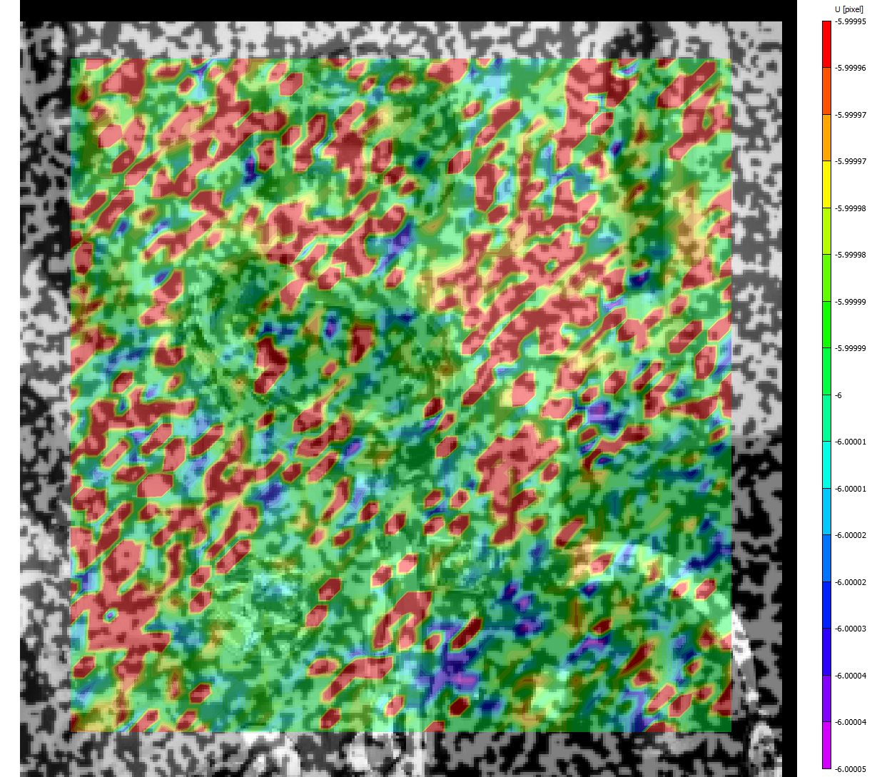
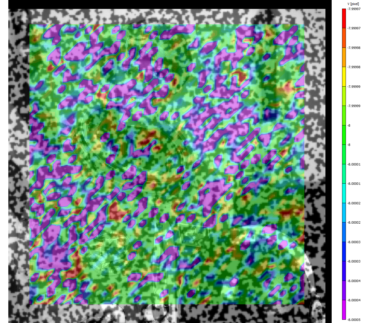
dx = -6, dy = 8 example (click either image for the full-size version): U, the x-axis displacement, uniformly -6 pixels (left, multi_point_motion_U); V, the y-axis displacement, uniformly -8 pixels (right, multi_point_motion_V) — VIC-2D's own -axis points opposite dictk's, so its sign is flipped from this page's dy = 8 even though both describe the identical physical motion.Across the 2861 subsets VIC-2D correlated successfully (109 more, all
along the image's outer edge, fell outside the shifted current image and
were masked out rather than reported), U ranges from exactly
to px and V from to px, in VIC-2D's own
columns (u_c/v_c in the raw output below). VIC-2D's own V
is measured with positive pointing up the page, opposite dictk's
downward-positive -axis. Once that sign difference is reconciled,
VIC-2D's result matches dictk's own / px ground truth exactly.
The full, subset-by-subset VIC-2D output,
multi_point_motion_vic_out.csv,
is available for closer inspection: every subset's position, displacement,
strain, and correlation quality metrics, not just the two summary fields
shown above. It carries two displacement column pairs: u_c/v_c
(VIC-2D's own convention, matching the two figures above exactly) and a
second u/v pair already expressed with v's sign flipped to match
dictk's downward-positive — u/v land on / px directly,
with no sign reconciliation needed to compare against dictk's ground
truth.
Next Steps
This page tracked rigid-body translation. Every point moved by the same amount. Simple Stretch is next. It tracks a stretching deformation, where each point moves by a different amount in the direction.