Continuum Mechanics
This section summarizes the kinematics of general (finite) motion, the motion map, the deformation gradient and its Jacobian, the family of finite-strain measures and their linearizations, and the polar and spectral decompositions.
- Upper case indices denote vector components in the reference configuration and
- Lower case indices denote vector components in the current configuration.
All vectors are referenced to origin and dextral, orthonormal basis vectors , , (equivalently, , , ).
Motion
Let the arbitrary time interval be defined as , from initial to final time, inclusive.1 Let the motion, a one-parameter family of configurations, , map the material particle (the reference configuration) into the current configuration ,
A motion evaluated at a particular time is referred to as a current configuration or placement. For any placement at time , there is a displacement field ,
Thus, the current configuration is simply a function of the original placement , plus a displacement , which is a function of reference configuration and time ,
The initial condition is found from the initial placement and the reference configuration ,
Deformation Gradient
To each configuration , we define a deformation gradient ,
Real, square matrices of dimension three with positive determinant are denoted . Gradient operations with and without a subscript "" are gradients taken in the reference and current configurations, respectively:
Alternative notations are and , respectively.
Jacobian of the Deformation Gradient
The Jacobian of the deformation gradient,
describes the (generally non-uniform) volumetric expansion or contraction of the motion from the reference configuration . All configurations must be admissible in the sense that the Jacobian of the deformation must be positive . This requirement keeps the deformations from mapping the body to a single, infinitesimally small point or turning the body inside-out .
Isochoric motions preserve the body's total volume. A Jacobian of unity describes an isochoric motion. The table below describes the categories of motions (expansion, volume-preserving, contraction, and inadmissible) by Jacobian measure.
| inadmissible | inadmissible | contraction | isochoric | expansion |
| body has turned inside-out | body has shrunk to zero volume | body's total volume has decreased | body's total volume is preserved | body's total volume has increased |
Four important isochoric deformations are (1) pure translation, (2) pure rotation, (3) isochoric stretch, and (4) isochoric shear.
Displacement Gradient
From the displacement field defined above, the relationship between the displacement gradient and the deformation gradient is given by
Right Cauchy-Green Deformation
The right Cauchy-Green deformation arises from the inner product of two differential fiber elements in the reference configuration, and , mapped by the deformation gradient to obtain the inner product of the same differential fibers in the current configuration, and ,
where
The right Cauchy-Green deformation tensor :
- is defined in the reference configuration,
- is symmetric and positive-definite,
- gets its name from the location of the deformation gradient in the definition, which is to the right,
- is a metric that maps fiber lengths from the reference configuration to the current configuration, and
- is second-order in reference displacement gradients, as shown below:
This result can be expected since, by definition, is second-order in the deformation gradient , and the relationship between the deformation gradient and the displacement gradient is linear.
Left Cauchy-Green Deformation
The left Cauchy-Green deformation arises from similar multiplication as with the right Cauchy-Green deformation, but with the stretching going in reverse, from the current configuration back to the reference configuration,
where
The left Cauchy-Green deformation tensor :
- is defined in the current configuration,
- is symmetric and positive-definite,
- gets its name from the location of the deformation gradient in the definition, which is to the left,
- is a metric whose inverse maps fiber lengths from the current configuration to the reference configuration, and
- is second-order in current displacement gradients.
Green-Lagrange Strain
The Green-Lagrange strain tensor,
is closely related to the right Cauchy-Green deformation tensor and is often used in defining constitutive law relationships because the measure, when linearized about the reference configuration, coincides with the small strain tensor of linear deformation elasticity, denoted and defined in the Infinitesimal Strain section. This relationship can be seen as follows:
where the higher-order (quadratic) term in the first line is set to zero to achieve the linearized second line.
Almansi-Euler Strain
The Almansi-Euler strain tensor,
can likewise be used to approximate the small strain tensor by combining the definitions of the left Cauchy-Green deformation and the deformation gradient as follows:
where the higher-order (quadratic) term is set to zero to achieve the linearized final line.
Small Strain
When displacement gradients are small in the reference configuration,
or in the current configuration,
respectively, the nonlinear gradient terms are negligible and the finite strain theory simplifies to small strain theory, which occurs when finite strain measures are linearized to obtain and in the previous sections.
Note that we have restricted the gradients of displacement, and not the displacement itself. Thus, displacements between the reference and current configurations can be large (finite), but the gradients of the displacement, either in the reference or current configuration, are small.
The Strain Tensors and Finite Rotations section will demonstrate that the small strain tensors are not suitable to describe motion that contains finite rotation. This makes sense because, in finite rotation, gradients of displacement are large, not small. To adequately describe motion that includes finite rotation, a fully nonlinear strain measure, such as the Seth-Hill strain family, must be used.
Infinitesimal Strain
If we further restrict the small strain theory such that the displacement is small compared to unity,
the infinitesimal strain theory is obtained, which has no distinction between Lagrangian and Eulerian strain tensors.
In this case, the two small strain tensors, and , converge to a single definition of strain, called the infinitesimal strain tensor , defined as
Note that the notation has been dropped since the distinction between the reference and current configurations is nonexistent. Also, note that the factor of appears because it then follows that the infinitesimal strain is simply the symmetric part of the displacement gradient,
Finally, note that the finite Lagrangian and Eulerian strain tensors were defined with the factor of so that their expressions, once linearized and subject to a small displacement assumption, simplify to exactly the infinitesimal strain tensor .
Seth-Hill Strain Family
We now return to finite strain definitions. Seth and Hill showed that the Green-Lagrange strain tensor and the Almansi-Euler strain tensor are special cases of the so-called Seth-Hill family of strain measures, defined as
The principal stretches , , allow the strain measure to be written as principal strains, as a function of principal stretch, ,
where the stretch function
For integer values2 of , five common strain measures result, listed in the table below, in their three-dimensional and one-dimensional forms. Similar relationships can be constructed for the spatial tensors using
| Name | 3D | 1D | |
|---|---|---|---|
| Green-Lagrange | |||
| engineering (Biot, nominal) | |||
| log (Hencky, natural) | |||
| true | |||
| Almansi-Euler |
The one-dimensional strains are illustrated as a function of stretch ratio in the figure below.
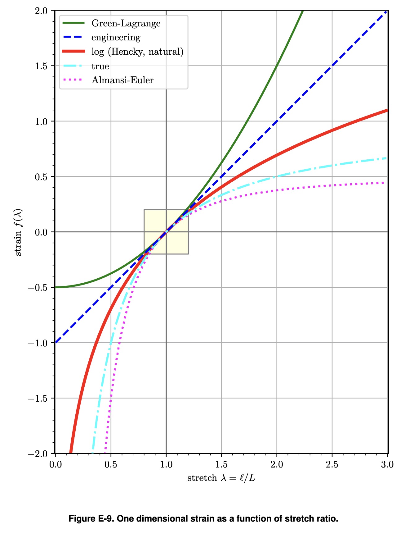
Source: Terpsma et al.3
The figure illustrates several results:
- For small stretches, , (a) the stretch ratio is near unity, , (b) the strain values are small, , and (c) the tangent of the strains with respect to the stretch ratio is near unity, .
- For elongations, , the strain monotonically increases since when .
- For extreme compressions, , (a) the Green-Lagrange strain goes to a value of , (b) the engineering (Biot, nominal) strain tensor goes to a value of , and (c) the log, true, and Eulerian strains tend to .
- The engineering (Biot, nominal) strain is a linear function of stretch ; all other measures are nonlinear functions of stretch .
Neff (2013)4 suggested "reasonable requirements" on , summarized in the table below, wherein a "+" indicates the requirement is satisfied and a "−" indicates the requirement is not satisfied.
| Requirement | |||||
|---|---|---|---|---|---|
| is smooth | + | + | + | + | + |
| is monotonically increasing | + | + | + | + | + |
| + | + | + | + | + | |
| + | + | + | + | + | |
| as , | + | + | + | − | − |
| as , | − | − | + | + | + |
| − | − | + | − | − | |
| for | − | − | + | − | − |
The results above illustrate that the log strain retains more of the desired qualities than any other strain tensor, in the context of finite compression and extension.5
- For infinitesimal deformation, all tensors converge to the infinitesimal strain tensor .
- For finite deformation, the Seth-Hill strain measures given by the function diverge quickly for both large compression and large tension.
The figure below illustrates the one-dimensional strains subtracted from the natural logarithmic strain, , as a function of stretch ratio . The log strain is considered as the finite deformation baseline.
The results show, for example, that in compression at , the Green-Lagrange strain tensor underreports the log strain by nearly 5%. Such a result illustrates that for finite deformation:
- Strain measures are not interchangeable, and
- It is ambiguous and incomplete to simply refer to "strain" as a deformation measure.
For finite deformation, both the strain value and the strain tensor must be specified.
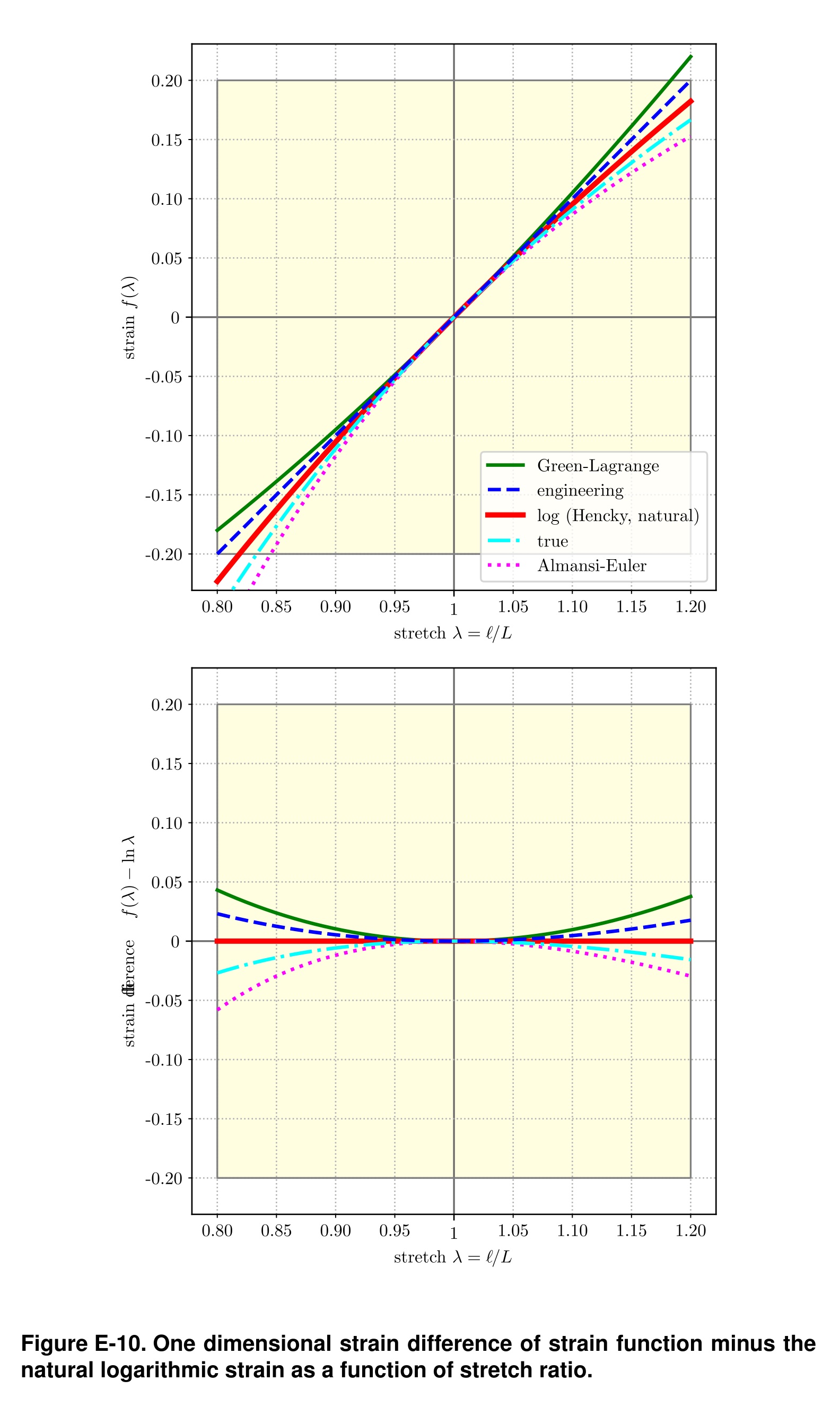
Source: Terpsma et al.3
Strain Tensors and Finite Rotations
Because it takes on nonzero values under finite rotation, the linearized strain tensor should not be used for geometrically nonlinear analysis. These nonzero values are completely artificial and strictly a result of using a linear strain definition with geometrically nonlinear motions. This result is shown as follows.
Let be a two-dimensional, rigid body rotation parameterized by time and scaled by constant radians per second. Then, the motion of a body can be written as
Then the deformation gradient is a function of time alone,
The linearized strain tensor is found to be
Now, for small angles, , which is for small deviations , , then for rigid body rotations. However, for arbitrary finite angles, , and the linearized strain tensor reports nonzero strain for rigid body rotations, which is nonsensical.
A correct strain tensor will report zero strain for rigid body rotations. One such strain tensor is the fully nonlinear Green-Lagrange strain tensor. This result is shown as follows:
Polar Decomposition
Given the rotation tensor , the material stretch tensor , and the spatial stretch tensor , the deformation gradient has the multiplicative decomposition,
Here we have a slight abuse of notation, where intermediate configurations that have stretched but not yet rotated are denoted with capital letter indices. Thus the "" subscript in is an intermediate stretched but non-rotated configuration.
The stretch tensors and are both symmetric and positive definite. The rotation tensor is non-symmetric and orthogonal. The figure below shows the polar decomposition about a material point and fibers in its vicinity mapped to the spatial point with the same fibers mapped to .
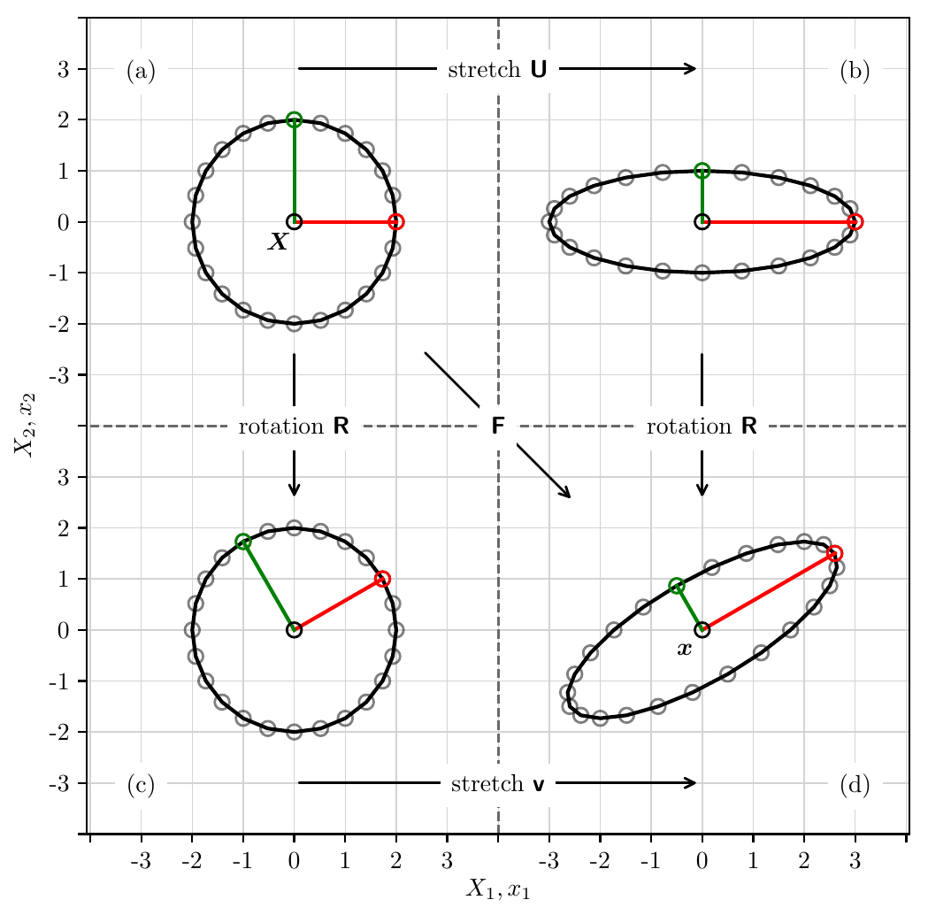
polar_decomposition.py.
Principal Stretches and Axes
The stretch tensors and have the same eigenvalues, , called principal stretches. For non-trivial rotations, i.e. , and have unique eigenvectors, called principal stretch directions. The principal stretch directions of are . The principal stretch directions of are . The two sets of eigenvectors are related through rotation ,
or generally,
Spectral Representation
The deformation gradient, its polar decomposition, and the Cauchy-Green deformations have spectral decompositions in terms of the principal stretches and stretch directions,
The Green-Lagrange strain tensor and the Almansi-Euler strain tensor , in principal stretches and stretch directions, are
The generalization of the Seth-Hill material strain tensor and spatial strain tensor , in principal stretches and stretch directions, are
and the relationship between the two strain tensors is given through a rotation transformation,
In the case when , the material and spatial logarithmic strain tensors, also known as the Hencky material and spatial strain tensors, and , are obtained as6
Two concrete illustrations follow: Rigid Body Motion works through pure translation as the simplest possible deformation, and Simple Shear works through an isochoric shear in closed form, computing , , , , and explicitly.
-
Note that , while typically zero, may be any real number less than . ↩
-
Technically, can be any real number, not just an integer. ↩
-
Terpsma RJ, Hovey CB. Blunt impact brain injury using cellular injury criterion. Sandia National Lab. (SNL-NM), Albuquerque, NM (United States); 2020 Oct 1. link ↩ ↩2
-
Neff, P. (2013). The Hencky strain measure is the geodesic distance to SO(), at 6. ↩
-
The Bažant strain, , not considered here, also satisfies . ↩
-
See Xiao H, Bruhns OT, Meyers A. Hypo-elasticity model based upon the logarithmic stress rate. Journal of Elasticity. 1997 Apr 1;47(1):51-68, at page 54, Eq. (2.2). ↩