Windowing

The FFT implicitly treats an image as one period of an infinitely-repeating signal. If the content doesn't tile seamlessly, which is the general case since nothing arranges an image's edges to match up, that discontinuity leaks energy across many frequencies rather than the few the underlying content actually has, an effect called spectral leakage. In a correlation surface, leakage broadens and can shift the peak, hurting the precision of any technique that searches that surface for a match.

Windowing counters this by tapering an image's edges toward zero before transforming it, so the (still discontinuous, but now near-zero) seam contributes far less energy. Two standard 1D windows, applied to an image by taking the outer product of a window with itself along each axis:

$$w_{\mathrm{Hann}}(n)=0.5\left(1-\cos \left(\frac{2\pi n}{N-1}\right)\right)$$

$$w_{\mathrm{Hamming}}(n)=0.54-0.46\cos \left(\frac{2\pi n}{N-1}\right)$$

for $n=0,\dots ,N-1$ across a window of length $N$. Hann tapers all the way to exactly zero at both ends; Hamming stops short (around $0.08$), trading a little residual discontinuity for a narrower main lobe in the transformed signal.

See Harris FJ. "On the use of windows for harmonic analysis with the discrete Fourier transform." Proceedings of the IEEE 1978;66(1):51-83. A U.S. government work, not protected by U.S. copyright.

window()

dictk.correlation.window applies either taper to a 2D array. This reuses kernel from Cross Correlation (CC) and the Fourier Domain section of Correlation Criteria — the same checkerboard0, p0, and kernel_margin — to show what tapering actually does to an image before it's passed to an FFT:

import numpy as np
import matplotlib.pyplot as plt
from dictk.image import read, PixelCoordinate, subimage, write
from dictk.correlation import window, WindowingMethod

reference_image = read(path="checkerboard0.png")
p0 = PixelCoordinate(x=100, y=75)
kernel_margin = 25
kernel = subimage(
    image=reference_image,
    origin=PixelCoordinate(x=p0.x - kernel_margin, y=p0.y - kernel_margin),
    width=2 * kernel_margin,
    height=2 * kernel_margin,
)
write(arr=kernel, path="windowing_kernel_original.png")

kernel_hann = window(arr=kernel, method=WindowingMethod.HANN)
write(arr=kernel_hann.astype(np.uint8), path="windowing_kernel_hann.png")

kernel_hamming = window(arr=kernel, method=WindowingMethod.HAMMING)
write(arr=kernel_hamming.astype(np.uint8), path="windowing_kernel_hamming.png")

# window()'s own weights, isolated from kernel's content: windowing an
# all-ones array leaves exactly the 2D weight array behind. A single row
# at the kernel's mid-height cuts through the row axis's own peak (~1.0),
# so what's left is each method's column-axis taper alone.
mid_row = kernel.shape[0] // 2
ones = np.ones_like(kernel, dtype=np.float64)
weight_profiles = {
    "none": np.ones(kernel.shape[1]),
    "hann": window(arr=ones, method=WindowingMethod.HANN)[mid_row, :],
    "hamming": window(arr=ones, method=WindowingMethod.HAMMING)[mid_row, :],
}
for name, profile in weight_profiles.items():
    fig, ax = plt.subplots(figsize=(4, 2.5), constrained_layout=True)
    ax.plot(profile, color="black")
    ax.set_ylim(-0.05, 1.05)  # shared across all three, for a fair comparison
    ax.set_xlabel("x (pixels)")
    ax.set_ylabel("window weight")
    fig.savefig(f"windowing_kernel_cut_{name}.png", dpi=300)
    plt.close(fig)

Saved: windowing_kernel_original.png, windowing_kernel_hann.png, windowing_kernel_hamming.png, windowing_kernel_cut_none.png, windowing_kernel_cut_hann.png, windowing_kernel_cut_hamming.png

none	Hann	Hamming

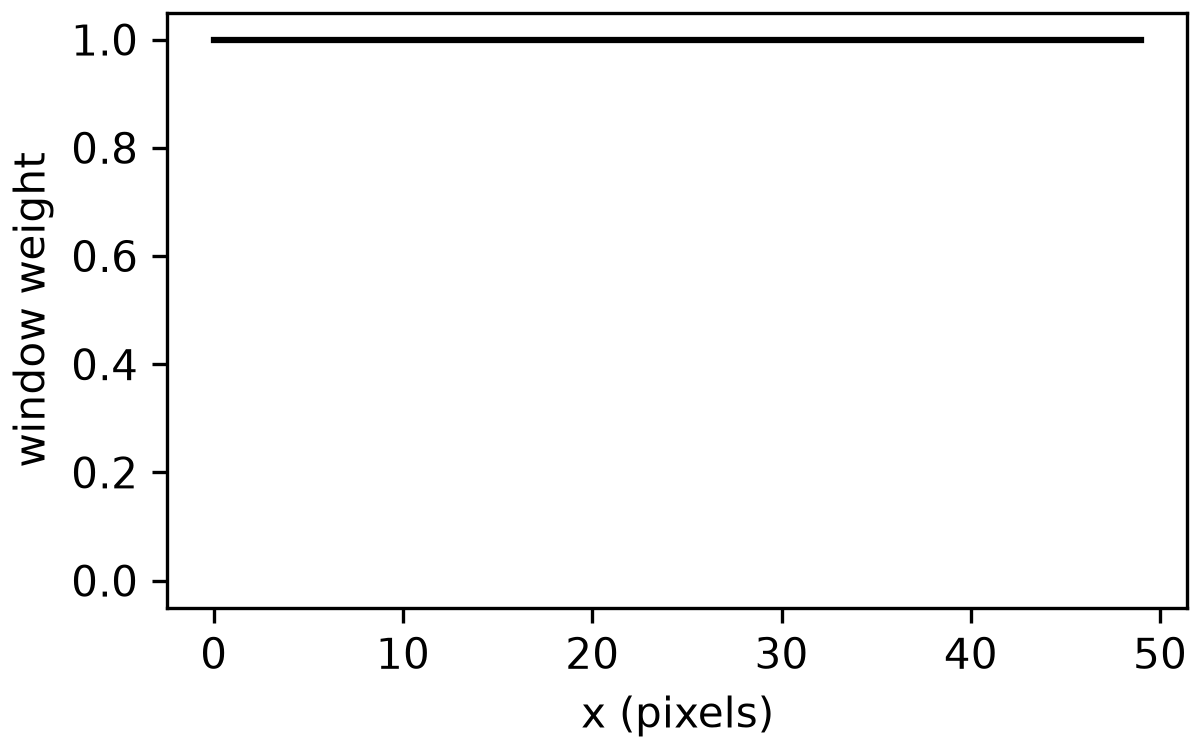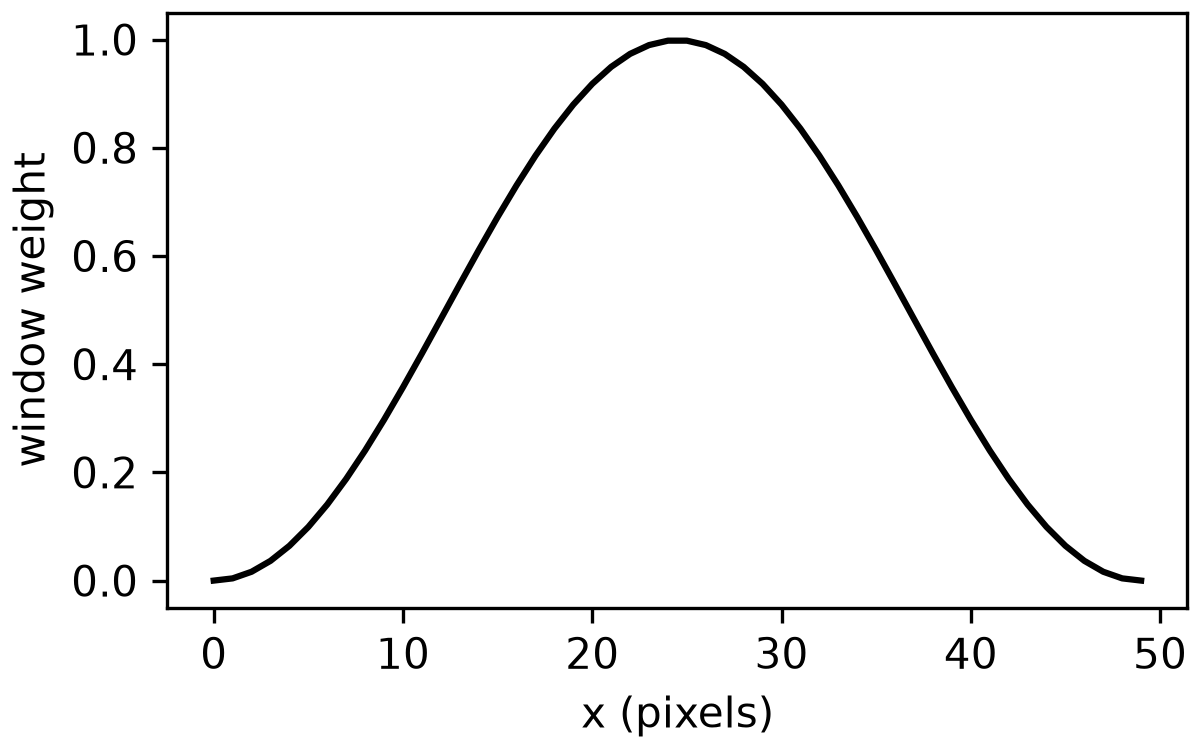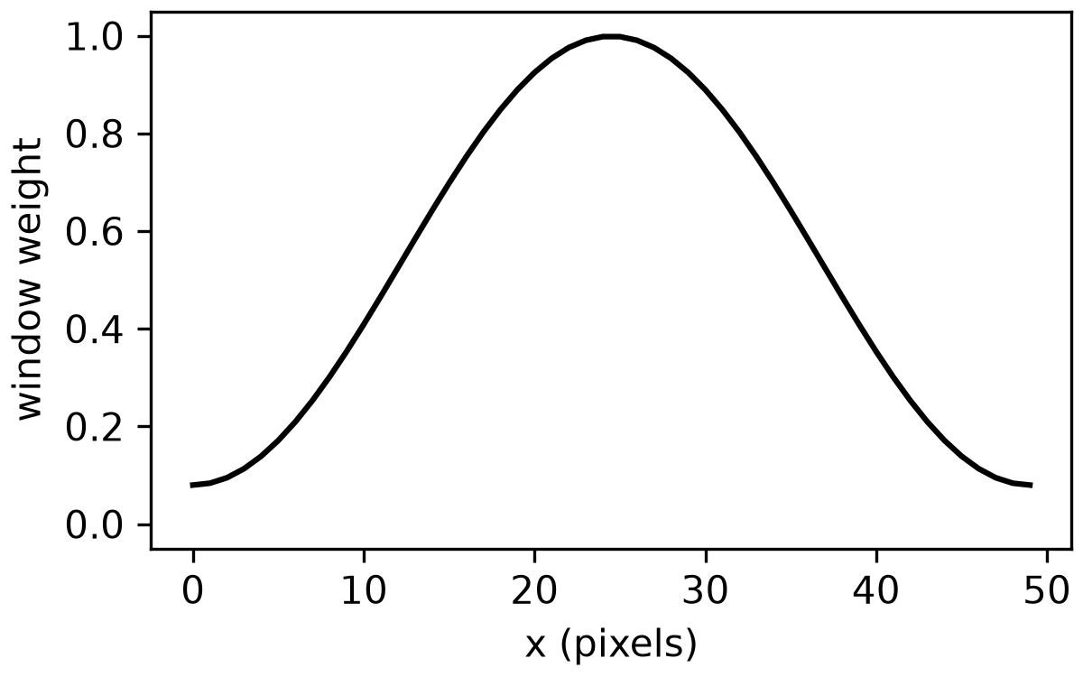Every edge fades toward black; Hann's corners go fully black (tapers to exactly 0), while Hamming's stay a faint gray (tapers to $0.08\times 0.08\approx 0.006$ of the original corner pixel, the product of both axes' own $0.08$ edge value).

The bottom row makes each method's own taper precise, independent of checkerboard0's content: a horizontal cut through the window's weight array at the kernel's mid-height, all three sharing the same $y$-axis. none is flat at $1.0$ everywhere -- no taper at all. Hann and Hamming both peak at $1.0$ at that same mid-height (the row axis's own window is near its own peak there), so this cut isolates the column axis's taper alone: Hann reaches exactly $0$ at both edges, Hamming levels off at $0.08$ -- not the smaller $0.006$ corner value above, since a corner is where both axes are simultaneously at their own edge, and a mid-height cut only ever passes through one axis's edge at a time.

See Correlation Visualization for windowing shown in action, tapering a real kernel and search area before they're compared.