Strain Window

Kernel Warping showed how dictk's locate_warp reduced the $E_{11}$ standard deviation for the 2% stretch to 1161 microstrain. locate_subpixel gave 16531 microstrain on the same stretch, and VIC-2D gave 1385 microstrain. Neither the locate_subpixel nor the locate_warp result used strain smoothing, the topic of this page. This page shows that strain smoothing reduces the strain error further.

Strain spread starts with tracking error. Every tracked point carries an error. A strain needs a derivative of displacement, and the derivative divides the error by the point spacing. For example, a 0.01 px error between two points 5 px apart puts 2000 microstrain ($0.01\text{px}/5\text{px}=0.002=2000$ microstrain) into the slope.

The Q4 elements behind the 1161 microstrain each differentiate across four neighboring points, 5 px apart. In contrast, a strain window differentiates across more points. It fits one plane to the displacements of every point in a square of neighboring points. The fit averages their errors, so the strain error drops. A 15x15-point window averages across 225 points.

The averaging has a cost. The plane assumes the strain is uniform across the window. If the real strain changes inside the window, the fit blurs that change into one number. Each point stands for a cell one spacing wide, so a window with $n$ points per side covers a side length of $n$ times the spacing. At 5 px point spacing:

• A 3x3 window averages 9 points and blurs over a side length of 15 px ($3\times 5$ px).
• A 15x15 window averages 225 points and blurs over a side length of 75 px ($15\times 5$ px).
• A 19x19 window averages 361 points and blurs over a side length of 95 px ($19\times 5$ px).

This page builds the strain window in three steps. In 1D, a row of three points shows the idea with three numbers. A 3x3 example then adds the second axis and gives the 2D result. Finally, a general window extends the 2D result to $n=2m+1$ points per side. At $m=1$, it recovers the 3x3 result. The page then compares the window's noise with the Q4 finite element's noise.

The Measured Result runs dictk.strain_window with a 15x15-point window on Kernel Warping's tracked positions:

• At the 1560 points with a full window, the $E_{11}$ standard deviation falls from 1161 microstrain to 39 microstrain.
• At all 2862 points (1560 full-window points + 1302 edge and corner points), the $E_{11}$ standard deviation falls from 1161 microstrain to 91 microstrain. The 1302 edge and corner points truncate their windows. Their spread alone is 117 microstrain.

Notation

In an image,

• $X$ runs across the page from left to right. The displacement $u$ points in the $X$ direction. Column $c$ grows from left to right.
• $Y$ runs down the page from top to bottom. The displacement $v$ points in the $Y$ direction. Row $r$ grows from top to bottom.

The steps below fit $u$. The fit for $v$ uses the same weights, as Fit for $v$ shows.

1D Example

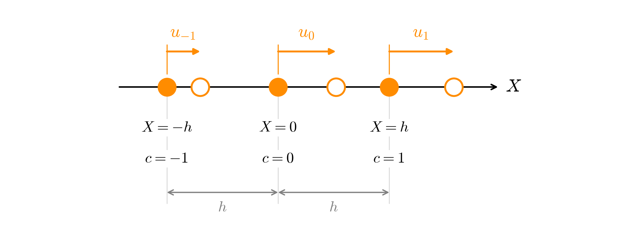
Consider three points on the $X$ axis. Index them by $c=-1,0,1$. Point $c$ sits at $X=ch$ relative to the middle point. The three points have tracked displacements $u_{-1}$, $u_0$, and $u_1$. Figure 10.1-1 shows the three points and their displacements.

Fit a straight line through the displacements. At $X=ch$, the line predicts

$$u_c\approx {\hat{u}}_0+\frac{\partial u}{\partial X}ch.\text{\hspace{1em}(10.1-1)}$$

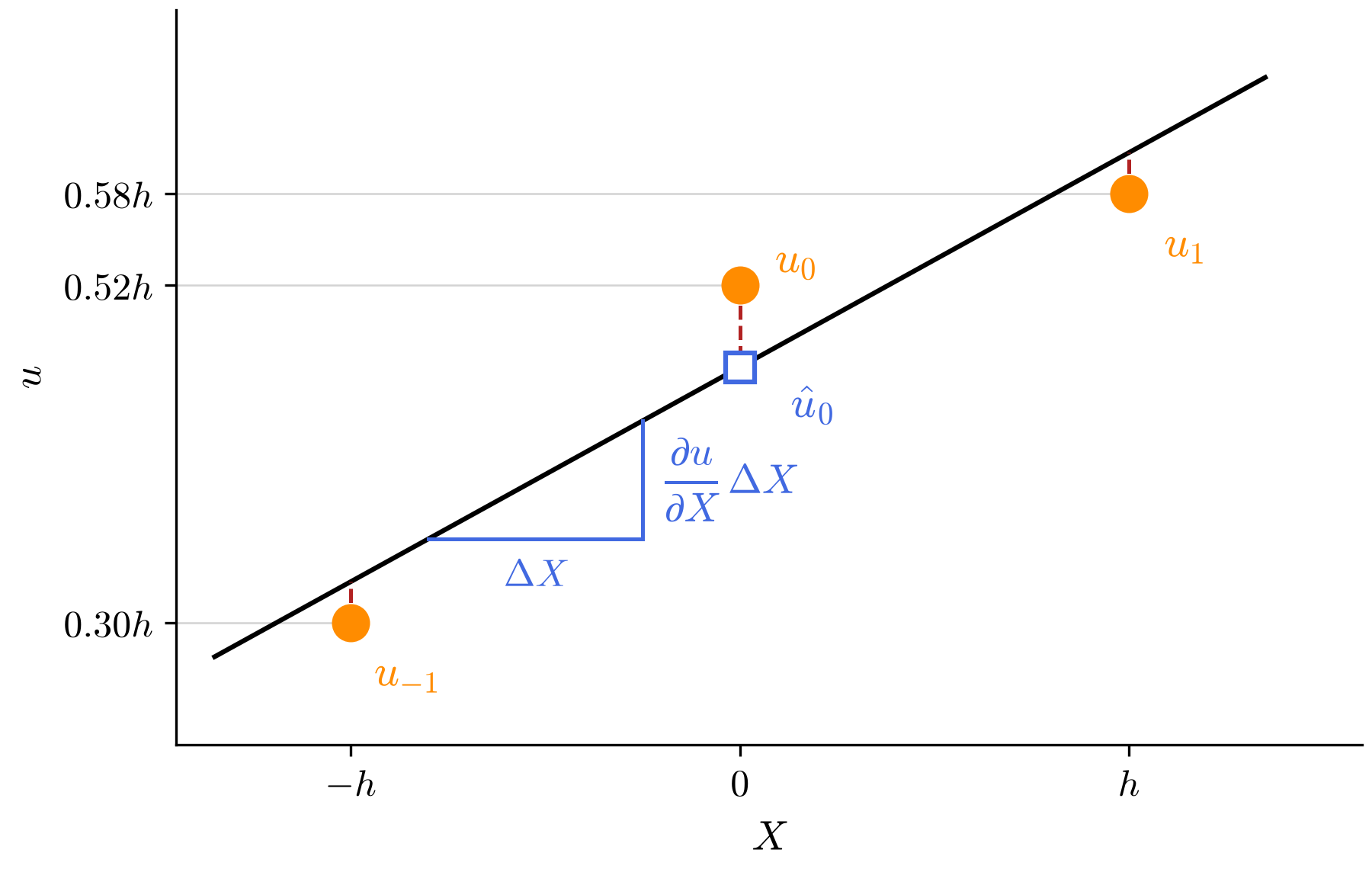
The slope of the line is $\partial u/\partial X$. The intercept of the line is ${\hat{u}}_0$, the fitted displacement at the middle point, where $c=0$. Figure 10.1-2 shows the line through the three displacements of Figure 10.1-1.

That is two unknowns, ${\hat{u}}_0$ and $\partial u/\partial X$, for three points. Least squares picks the two unknowns that minimize the sum of the three squared residuals:

$$\begin{array}{rl}R& =\sum _{c=-1}^1{\left(u_c-{\hat{u}}_0-\frac{\partial u}{\partial X}ch\right)}^2\\ & ={\left(u_{-1}-{\hat{u}}_0+\frac{\partial u}{\partial X}h\right)}^2+{\left(u_0-{\hat{u}}_0\right)}^2+{\left(u_1-{\hat{u}}_0-\frac{\partial u}{\partial X}h\right)}^2.\end{array}$$

At the minimum, the derivative of $R$ with respect to each unknown is zero. The derivative with respect to ${\hat{u}}_0$ is

$$\frac{\partial R}{\partial {\hat{u}}_0}=-2\sum _c\left(u_c-{\hat{u}}_0-\frac{\partial u}{\partial X}ch\right)=0.$$

Rearranged, that gives the first normal equation:

$${\hat{u}}_0\sum _{c}1+\frac{\partial u}{\partial X}h\sum _{c}c=\sum _c{u}_c.$$

The derivative with respect to the slope $\partial u/\partial X$ is

$$\frac{\partial R}{\partial (\partial u/\partial X)}=-2\sum _{c}ch\left(u_c-{\hat{u}}_0-\frac{\partial u}{\partial X}ch\right)=0.$$

Dividing by $-2$ and rearranging gives the second normal equation:

$${\hat{u}}_{0}h\sum _{c}c+\frac{\partial u}{\partial X}{h}^2\sum _c{c}^2=h\sum _{c}c{u}_c.$$

In matrix form, the two normal equations are

$$\left[\begin{array}{cc}{\sum }_{c}1& h{\sum }_{c}c\\ h{\sum }_{c}c& h^2{\sum }_c{c}^2\end{array}\right]\left\{\begin{array}{c}{\hat{u}}_0\\ \partial u/\partial X\end{array}\right\}=\left\{\begin{array}{c}{\sum }_c{u}_c\\ h{\sum }_{c}c{u}_c\end{array}\right\}.$$

The sums are ${\sum }_{c}1=3$, ${\sum }_{c}c=-1+0+1=0$, and ${\sum }_c{c}^2=1+0+1=2$. So the matrix is

$$\left[\begin{array}{cc}3& 0\\ 0& 2h^2\end{array}\right].$$

The zero off the diagonal decouples the two unknowns:

$$\boxed{\begin{array}{rl}{\hat{u}}_0& =\frac{u_{-1}+u_0+u_1}{3},\\ \frac{\partial u}{\partial X}& =\frac{h(-u_{-1}+u_1)}{2h^2}=\frac{u_1-u_{-1}}{2h}.\end{array}}\text{\hspace{1em}(10.1-2)}$$

The slope is the central difference. The middle point gets zero weight in it.

Noise

How much does tracking error move the slope? Work it out in six steps.

Step 1: model the error. Each tracked displacement is the true displacement plus an error:

$$u_c=u_c^{\text{true}}+e_c.$$

The three errors $e_{-1}$, $e_0$, and $e_1$ are independent. Each has mean 0 and standard deviation $\sigma$, so each has variance ${\sigma }^2$.

Step 2: find the error in the slope. Substitute step 1 into the slope:

$$\frac{\partial u}{\partial X}=\frac{u_1-u_{-1}}{2h}=\underset{\text{true slope}}{\underbrace{\frac{u_1^{\text{true}}-u_{-1}^{\text{true}}}{2h}}}+\underset{\text{slope error}}{\underbrace{\frac{e_1-e_{-1}}{2h}}}.$$

The true part has no randomness. So the slope's variance is the variance of the slope error alone. The middle point's error $e_0$ does not appear, because the middle point has zero weight.

Step 3: recall two variance rules. For a constant $\alpha$ and independent errors $e_a$ and $e_b$:

$$\begin{array}{rl}\mathrm{Var}(\alpha e_a)& ={\alpha }^2\mathrm{Var}(e_a),\\ \mathrm{Var}(e_a\pm e_b)& =\mathrm{Var}(e_a)+\mathrm{Var}(e_b).\end{array}$$

Variances add for a difference too, because the sign flips with $\alpha =-1$ and ${\alpha }^2=1$.

Step 4: apply the first rule to each term. The slope error has two terms, $e_1/2h$ and $-e_{-1}/2h$. Each one is an error scaled by $\alpha =\pm 1/(2h)$:

$$\mathrm{Var}\left(\frac{e_1}{2h}\right)=\mathrm{Var}\left(\frac{-e_{-1}}{2h}\right)=\frac{{\sigma }^2}{4h^2}.$$

Step 5: apply the second rule to add them.

$$\mathrm{Var}\left(\frac{\partial u}{\partial X}\right)=\frac{{\sigma }^2}{4h^2}+\frac{{\sigma }^2}{4h^2}=\frac{{\sigma }^2}{2h^2}.$$

Step 6: take the square root. The standard deviation is

$$\mathrm{std}\left(\frac{\partial u}{\partial X}\right)=\frac{\sigma }{\sqrt{2}h}=0.707\frac{\sigma }{h}.\text{\hspace{1em}(10.1-3)}$$

For example, take $\sigma =0.01$ px and $h=5$ px. The slope's standard deviation is $0.707\times 0.01/5=0.00141$, or 1414 microstrain.

A slope's noise reads as strain noise because, at small strain, $E_{11}\approx \partial u/\partial X$. For a uniaxial stretch, $E_{11}=\ln (1+\partial u/\partial X)$, so $d{E}_{11}/d(\partial u/\partial X)=1/(1+\partial u/\partial X)$. At the 2% stretch on these pages, that factor is $1/1.02=0.98$. So log strain noise runs 2% below slope noise. This page quotes slope noise. From Gradient to Strain gives the full chain from slopes to strain.

The slope uses only 2 of the 3 points. The 3x3 window below averages three such rows. Before the 3x3 result, Q4 Baseline derives a Q4 element's noise for comparison in 2D.

Q4 Baseline

Finite Element Method computes strain from Q4 elements. Every strain on the earlier pages comes from them. This section derives a Q4 element's noise. The window sections below compare against it, for two reasons.

• Q4 is the method dictk uses now. Kernel Warping measured its 1161 microstrain spread with gauss_point_log_strains, which evaluates Q4 elements. A window must beat that to earn a place in dictk.
• Q4 sets the unit of improvement. The 1D slope's noise scales with $\sigma /h$. The Q4 element's and the window's do too. One number for each turns every comparison into a ratio.

Gauss-Point Gradient

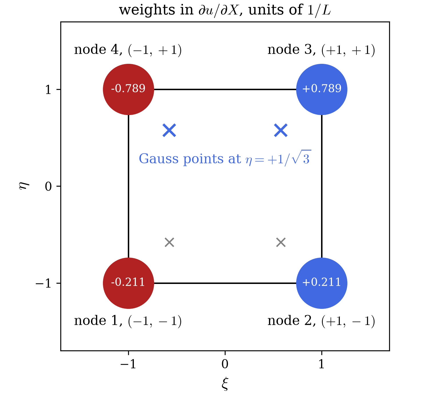
Take a square Q4 element with side $L$. Its nodes 1 to 4 sit at $(\xi ,\eta )=(-1,-1)$, $(1,-1)$, $(1,1)$, and $(-1,1)$. At the two Gauss points with $\eta =+1/\sqrt{3}$, its gradient is

$$\begin{array}{rl}\frac{\partial u}{\partial X}& =\frac{1}{L}\left[g_1(u_2-u_1)+g_2(u_3-u_4)\right],\\ g_{1,2}& =\frac{1\mp 1/\sqrt{3}}{2}.\end{array}\text{\hspace{1em}(10.1-4)}$$

So $g_1=0.211$ and $g_2=0.789$. The edge nearer the Gauss point gets the larger weight. The two Gauss points at $\eta =-1/\sqrt{3}$ swap $g_1$ and $g_2$. Figure 10.1-3 shows the weights. The script computes them with dictk.element.

Q4 Noise

The weights satisfy $g_1+g_2=1$ and $g_1^2+g_2^2=2/3$. Each node enters once, with weight $\pm g_1/L$ or $\pm g_2/L$. The variance rules from the 1D Example's Noise give

$$\mathrm{std}\left(\frac{\partial u}{\partial X}\right)=\frac{\sigma }{L}\sqrt{2\left(g_1^2+g_2^2\right)}=\frac{2}{\sqrt{3}}\frac{\sigma }{L}=1.155\frac{\sigma }{L}.\text{\hspace{1em}(10.1-5)}$$

All four Gauss points give the same value, because each one uses the same four weights in a different order.

The earlier pages build each Q4 element from 4 neighboring tracked points, so $L=h$. The standard deviation is then $1.155\sigma /h$. For $\sigma =0.01$ px and $h=5$ px, that is 2309 microstrain. The 1D Example's central difference gives 1414 microstrain at the same $\sigma$ and $h$. The 2D Example compares the 3x3 window with both.

2D Example

The smallest square window with a center point holds 3x3 = 9 points. It is the general window with $m=1$.

Setup

The points sit on a grid with spacing $h$. Point $(c,r)$ sits at $X=ch$ and $Y=rh$ relative to the center point $(0,0)$. The window fits a plane through the 9 tracked displacements:

$$u_{c,r}\approx {\hat{u}}_0+\frac{\partial u}{\partial X}ch+\frac{\partial u}{\partial Y}rh.\text{\hspace{1em}(10.1-6)}$$

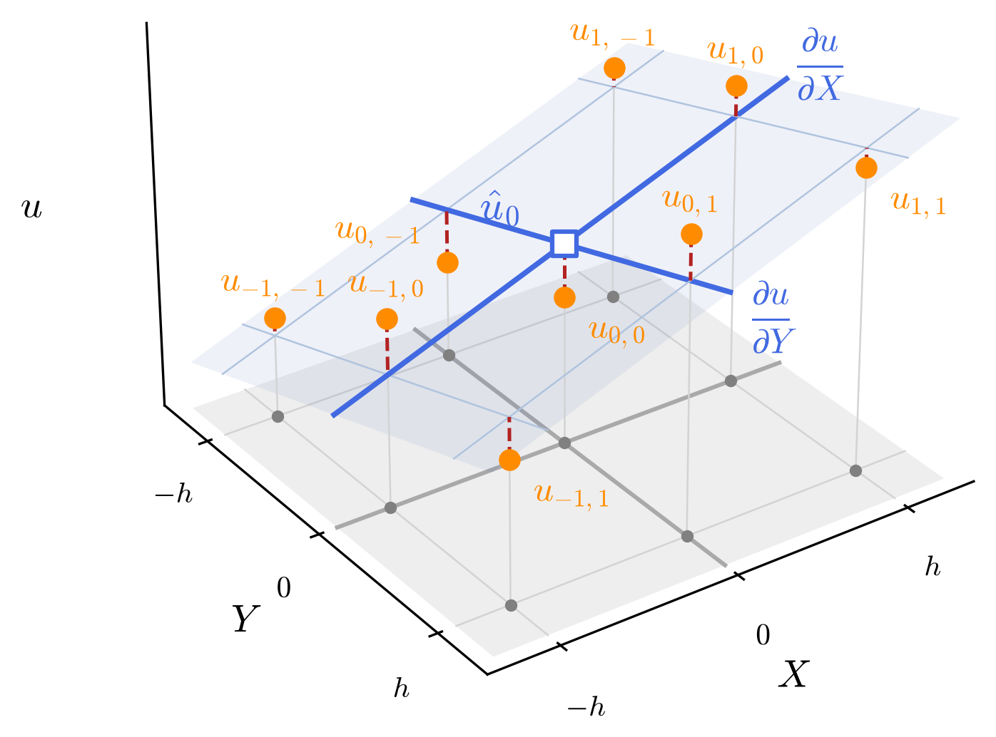
That is three unknowns, ${\hat{u}}_0$, $\partial u/\partial X$, and $\partial u/\partial Y$, for nine points. Figure 10.1-4 shows the plane through nine displacements. It extends Figure 10.1-2 from a line to a plane.

Normal Equations

Least squares minimizes the sum of the nine squared residuals:

$$R=\sum _{c=-1}^1\sum _{r=-1}^1{\left(u_{c,r}-{\hat{u}}_0-\frac{\partial u}{\partial X}ch-\frac{\partial u}{\partial Y}rh\right)}^2.$$

As in the 1D Example, each derivative of $R$ is zero at the minimum. Write ${\hat{e}}_{c,r}$ for the residual inside the parentheses. The three derivatives are

$$\begin{array}{rl}\frac{\partial R}{\partial {\hat{u}}_0}& =-2\sum _{c,r}{\hat{e}}_{c,r}=0,\\ \frac{\partial R}{\partial (\partial u/\partial X)}& =-2\sum _{c,r}ch{\hat{e}}_{c,r}=0,\\ \frac{\partial R}{\partial (\partial u/\partial Y)}& =-2\sum _{c,r}rh{\hat{e}}_{c,r}=0.\end{array}$$

Dividing each by $-2$ and rearranging gives three normal equations. In matrix form, they are

$$\left[\begin{array}{ccc}\sum 1& h\sum c& h\sum r\\ h\sum c& h^2\sum c^2& h^2\sum cr\\ h\sum r& h^2\sum cr& h^2\sum r^2\end{array}\right]\left\{\begin{array}{c}{\hat{u}}_0\\ \partial u/\partial X\\ \partial u/\partial Y\end{array}\right\}=\left\{\begin{array}{c}\sum u_{c,r}\\ h\sum c{u}_{c,r}\\ h\sum r{u}_{c,r}\end{array}\right\}.\text{\hspace{1em}(10.1-7)}$$

Each sum runs over the 9 points:

• $\sum 1=9$.
• $\sum c=0$. Three points sit at each of $c=-1$, $0$, and $1$, so they cancel. $\sum r=0$ for the same reason.
• $\sum cr=0$. Flipping $c$ to $-c$ flips the product's sign, so the points cancel in pairs.
• $\sum c^2=3+0+3=6$. $\sum r^2=6$ for the same reason.

So the matrix is

$$\left[\begin{array}{ccc}9& 0& 0\\ 0& 6h^2& 0\\ 0& 0& 6h^2\end{array}\right].$$

The matrix is diagonal, so each equation holds only one unknown.

Solution

Each unknown divides one right-side entry by one diagonal entry:

$$\boxed{\begin{array}{rl}{\hat{u}}_0& =\frac{1}{9}\sum _{c,r}{u}_{c,r},\\ \frac{\partial u}{\partial X}& =\frac{h\sum c{u}_{c,r}}{6h^2}=\frac{1}{6h}\sum _{c,r}c{u}_{c,r},\\ \frac{\partial u}{\partial Y}& =\frac{h\sum r{u}_{c,r}}{6h^2}=\frac{1}{6h}\sum _{c,r}r{u}_{c,r}.\end{array}}\text{\hspace{1em}(10.1-8)}$$

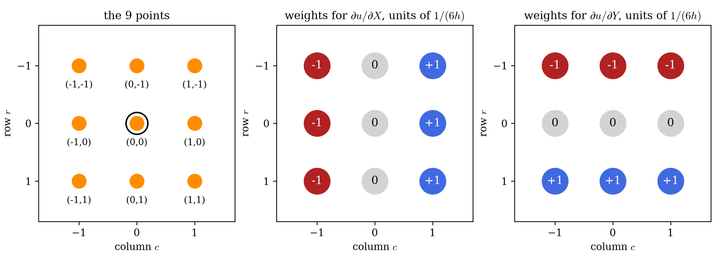
Figure 10.1-5 draws the weights. In $\partial u/\partial X$, the right column enters with $+1$, the left column with $-1$, and the middle column with 0. Group the sum by row. Each row contributes $u_{1,r}-u_{-1,r}$. In $\partial u/\partial Y$, the bottom row enters with $+1$, the top row with $-1$, and the middle row with 0. Group that sum by column. Each column contributes $u_{c,1}-u_{c,-1}$. So

$$\begin{array}{rl}\frac{\partial u}{\partial X}& =\frac{1}{3}\sum _{r=-1}^1\frac{u_{1,r}-u_{-1,r}}{2h},\\ \frac{\partial u}{\partial Y}& =\frac{1}{3}\sum _{c=-1}^1\frac{u_{c,1}-u_{c,-1}}{2h}.\end{array}$$

• $\partial u/\partial X$ is the mean of three central differences, one per row. The window differentiates along $X$ and averages along $Y$.
• $\partial u/\partial Y$ is the mean of three central differences, one per column. The window differentiates along $Y$ and averages along $X$.

Fit for $v$

Every entry of the matrix in the normal equations is a sum over $c$, $r$, and $h$. No entry holds a displacement. So the fit for $v$ uses the same matrix. Only the right side changes, from $u_{c,r}$ to $v_{c,r}$. The same diagonal entries give

$$\boxed{\begin{array}{rl}{\hat{v}}_0& =\frac{1}{9}\sum _{c,r}{v}_{c,r},\\ \frac{\partial v}{\partial X}& =\frac{1}{6h}\sum _{c,r}c{v}_{c,r},\\ \frac{\partial v}{\partial Y}& =\frac{1}{6h}\sum _{c,r}r{v}_{c,r}.\end{array}}\text{\hspace{1em}(10.1-9)}$$

The weights match Figure 10.1-5. They multiply $v$ instead of $u$.

Noise in the 3x3 Window

The solution writes $\partial u/\partial X$ as a weighted sum $\sum w_{c,r}^X{u}_{c,r}$ with $w_{c,r}^X=c/(6h)$. Independent errors give

$$\mathrm{Var}\left(\frac{\partial u}{\partial X}\right)={\sigma }^2\sum _{c,r}{\left(w_{c,r}^X\right)}^2={\sigma }^2\frac{6}{(6h{)}^2}=\frac{{\sigma }^2}{6h^2}.\text{\hspace{1em}(10.1-10)}$$

The standard deviation is $\sigma /(\sqrt{6}h)=0.408\sigma /h$. The row of three points gave $0.707\sigma /h$. Averaging three independent rows divides that by $\sqrt{3}$, and $0.707/\sqrt{3}=0.408$.

The weights for $\partial u/\partial Y$ are $r/(6h)$. Their squares sum to the same $6/(6h{)}^2$, so $\partial u/\partial Y$ also has standard deviation $0.408\sigma /h$. The fit for $v$ uses the same weights. If the errors in $v$ have the same $\sigma$, $\partial v/\partial X$ and $\partial v/\partial Y$ have $0.408\sigma /h$ too.

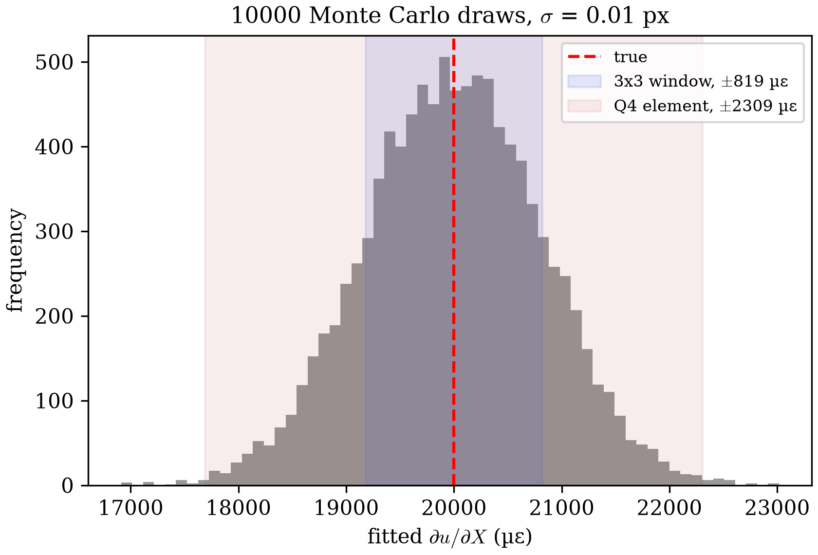
A Monte Carlo simulation checks the formula. The grid spacing is $h=5$ px. The true field has ${\hat{u}}_0=0.3$ px, $\partial u/\partial X=0.02$, and $\partial u/\partial Y=0.01$. Each of 10,000 draws adds an independent Gaussian error with $\sigma =0.01$ px to all 9 displacements, with random seed 0. That $\sigma$ is illustrative. It is not measured from a tracker. A tracker's errors also correlate between neighboring points, as Noise in a General Window shows.

The formula gives 816 microstrain. The 10,000 Monte Carlo draws give 819 microstrain. A Q4 element gives 2309 microstrain, 2.8 times more. Q4 Noise derives that value.

Figure 10.1-6 shows the 10,000 fitted slopes.

General Window

A general window holds $n\times n$ points, with $n=2m+1$. The steps match the 3x3 window's. Each result reduces to the 3x3 result at $m=1$.

Setup

Columns $c$ and rows $r$ each run from $-m$ to $m$. The fit is the same plane:

$$u_{c,r}\approx {\hat{u}}_0+\frac{\partial u}{\partial X}ch+\frac{\partial u}{\partial Y}rh.$$

That is three unknowns for $n^2$ points. For $n=15$ and $h=5$ px, the window holds 225 points. Its extent is $nh=75$ px, because each point stands for a cell $h$ wide. The two outermost points sit $(n-1)h=70$ px apart. This page uses the extent $nh$ for the region a window blurs over, and the outer-point distance $(n-1)h$ for the footprint that Window versus Q4 compares with a Q4 element.

Normal Equations

The residual sum $R$, its derivatives, and the matrix form match the 3x3 window's. Only the limits change: every sum now runs from $-m$ to $m$. One sum appears repeatedly. Call it $S_m$:

$$S_m=\sum _{c=-m}^m{c}^2=\frac{m(m+1)(2m+1)}{3}.\text{\hspace{1em}(10.1-11)}$$

The window's sums follow from it:

• $\sum 1=n^2$.
• $\sum c=\sum r=\sum cr=0$, by the same cancellations as the 3x3 window.
• $\sum c^2=n{S}_m$, because each of the $n$ rows contributes $S_m$. $\sum r^2$ is the same.

So the matrix is

$$\left[\begin{array}{ccc}{n}^2& 0& 0\\ 0& h^{2}n{S}_m& 0\\ 0& 0& h^{2}n{S}_m\end{array}\right].$$

At $m=1$: $n=3$ and $S_1=2$, so the diagonal is $(9,6h^2,6h^2)$.

Solution

$$\boxed{\begin{array}{rl}{\hat{u}}_0& =\frac{1}{n^2}\sum _{c,r}{u}_{c,r},\\ \frac{\partial u}{\partial X}& =\frac{h\sum c{u}_{c,r}}{h^{2}n{S}_m}=\sum _{c,r}{w}_{c,r}^X{u}_{c,r},\\ \frac{\partial u}{\partial Y}& =\frac{h\sum r{u}_{c,r}}{h^{2}n{S}_m}=\sum _{c,r}{w}_{c,r}^Y{u}_{c,r},\\ {\hat{v}}_0& =\frac{1}{n^2}\sum _{c,r}{v}_{c,r},\\ \frac{\partial v}{\partial X}& =\sum _{c,r}{w}_{c,r}^X{v}_{c,r},\\ \frac{\partial v}{\partial Y}& =\sum _{c,r}{w}_{c,r}^Y{v}_{c,r},\\ w_{c,r}^X& =\frac{c}{hn{S}_m},\\ w_{c,r}^Y& =\frac{r}{hn{S}_m}.\end{array}}\text{\hspace{1em}(10.1-12)}$$

At $m=1$, the weights are $w_{c,r}^X=c/(6h)$ and $w_{c,r}^Y=r/(6h)$.

The weight grows linearly with $c$. The outermost columns, at $c=\pm m$, carry the largest weights. A displacement $mh$ from the center changes by $mh$ times any change in slope, so it gets $m$ times the weight of a point at $c=\pm 1$. The weight does not depend on $r$. So the estimator fits one line per row and averages the $n$ row slopes. Figure 10.1-7 shows the weights for $m=1$, 2, and 3. The script also solves the normal equations directly and compares:

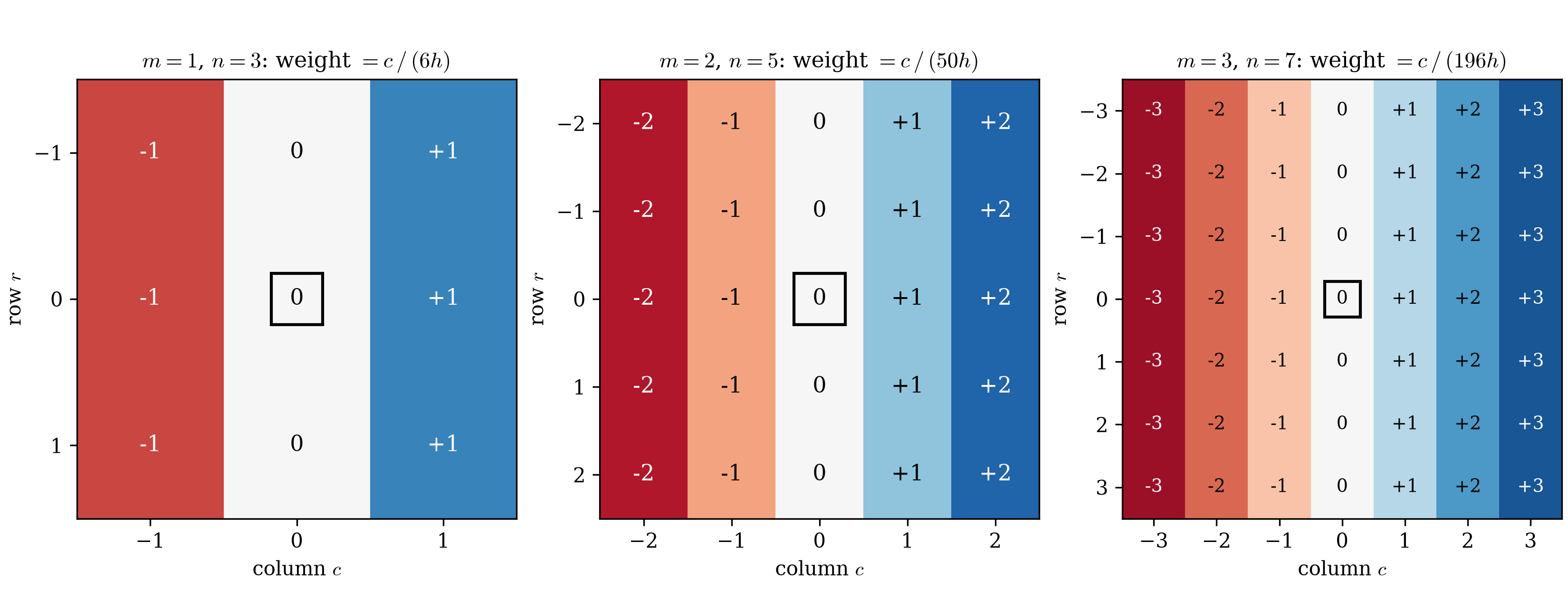
The weights depend only on $m$ and $h$. They do not depend on the images. So one set of weights serves every interior window, and for both $u$ and $v$.

Noise in a General Window

Independent errors give

$$\mathrm{Var}\left(\frac{\partial u}{\partial X}\right)={\sigma }^2\sum _{c,r}{\left(w_{c,r}^X\right)}^2={\sigma }^2\frac{n{S}_m}{(hn{S}_m{)}^2}=\frac{{\sigma }^2}{h^{2}n{S}_m}=\frac{3{\sigma }^2}{h^2{n}^{2}m(m+1)}.$$

The standard deviation is

$$\mathrm{std}\left(\frac{\partial u}{\partial X}\right)=\frac{\sigma }{h}\cdot \frac{1}{n}\sqrt{\frac{3}{m(m+1)}}\approx \frac{\sqrt{12}\sigma }{h{n}^2}\text{for large }m.\text{\hspace{1em}(10.1-13)}$$

At $m=1$, it is $\sigma /(\sqrt{6}h)$. The standard deviation falls as $n^{-2}$. Each row's line fit contributes $n^{-3/2}$. A row has $n$ points, and its outer points sit $mh$ from the center, so $S_m$ grows as $m^3$. Averaging the $n$ rows contributes the remaining $n^{-1/2}$.

The table compares the formula with a Monte Carlo simulation of 4000 random draws per window and with the Q4 element's $1.155\sigma /h$. Figure 10.1-8 plots the same comparison for $n$ from 3 to 19:

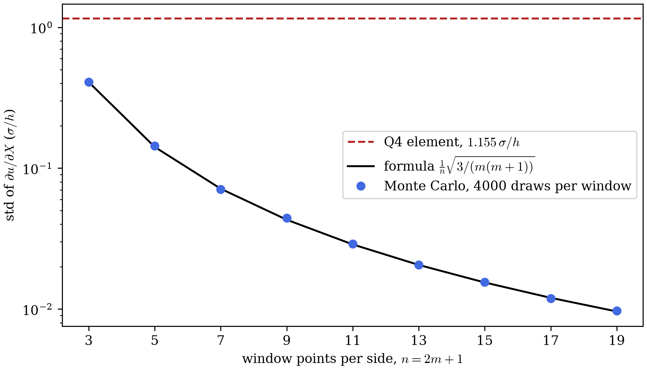
If the tracking errors were independent, the $74.8\times$ reduction at $n=15$ would cut Kernel Warping's 1161 microstrain to 15.5 microstrain. That $74.8\times$ compares the window with a Q4 element on the same grid. Window versus Q4 splits it by source.

Measured Result measures 39 microstrain at the interior points, 2.5 times more. The tracking error is not independent. Kernel Warping found a wave with a 51 px period. Points 5 px apart sit 35° apart on that wave's cycle, so their errors correlate at $\cos 35°=0.82$. Frequency Response computes the fraction of a wave's slope that a window passes.

Uniform Weights

Every point here gets the same weight in the sum of squared residuals. For independent errors with equal variance, uniform weights give the lowest variance of any linear unbiased estimator. A tent or Gaussian weight would reduce the influence of each window's outer points. Both are candidate refinements for a later stage. Neither appears here.

Window versus Q4

Q4 Baseline derived a Q4 element's noise, $1.155\sigma /L$. Noise in a General Window derived the window's. This section compares the two at any window size. Two points frame the comparison.

• Q4 shows where the gain comes from. A Q4 element fits 4 coefficients to 4 displacements. The fit is exact, so it averages nothing. A 15x15 window fits 3 coefficients to 225 displacements. That redundancy does the averaging.
• A fair comparison controls for footprint. On a grid with spacing $h$, a Q4 element spans $h$. A 15x15 window spans $14h$ between its outer points. That larger footprint alone accounts for $14\times$ of the window's $74.8\times$ lead. It also blurs the strain field. Equal Footprint holds the footprint fixed. Q4 at Equal Resolution holds the resolution fixed, which is the fairer test.

Equal Spacing

A Q4 element at $L=h$ gives 2309 microstrain. The 3x3 window gives 816 microstrain, 2.8 times less, at the same $\sigma =0.01$ px and $h=5$ px. Dividing the Q4 standard deviation by the general window's standard deviation gives the ratio for any window size:

$$\frac{{\mathrm{std}}_{\text{Q4}}}{{\mathrm{std}}_{\text{window}}}=\frac{2n\sqrt{m(m+1)}}{3}.\text{\hspace{1em}(10.1-14)}$$

The ratio is 2.8 at $m=1$ and 74.8 at $m=7$. It gives the gain dictk would see by replacing its Q4 elements with windows on the same grid. It does not split that gain by source.

Equal Footprint

A 15x15 window at $h=5$ px spans 70 px between its outer points. A Q4 element at $L=h$ spans 5 px. To remove the footprint gain, give the Q4 element the window's footprint. Its corners then sit on the window's 4 corner points, and $L=2mh$. Figure 10.1-9 shows the three choices on one grid.

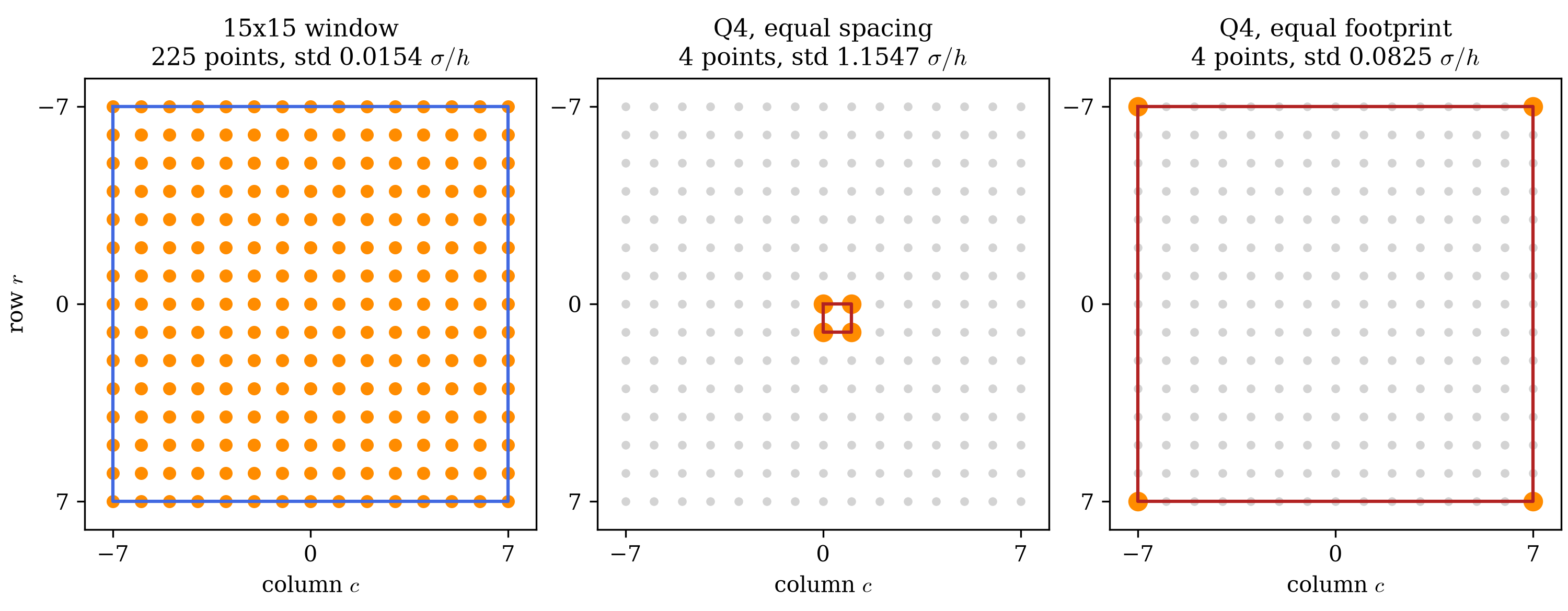
With $L=2mh$, the ratio becomes

$$\frac{{\mathrm{std}}_{\text{Q4}}}{{\mathrm{std}}_{\text{window}}}=\frac{n\sqrt{m(m+1)}}{3m}.\text{\hspace{1em}(10.1-15)}$$

The ratio is 1.41 at $m=1$ and 5.35 at $m=7$, and it approaches $n/3$ as $m$ grows. The two ratios differ by exactly $2m$, the ratio of the footprints. At $n=15$, $74.8=14\times 5.35$. The 14 comes from the footprint. The 5.35 comes from the fit. The window fits 225 displacements by least squares. The Q4 element interpolates 4 exactly.

Counting points alone suggests $\sqrt{225/4}=7.5\times$. Two effects turn that into $5.35\times$. First, the window's interior points sit closer to its center. A change in slope moves a point in column $c$ by an amount proportional to $c$. So each point adds information about the slope in proportion to $c^2$. A point at $c=1$ adds 1/49 as much as a point at $c=7$. The 15 points at $c=0$ add none. Over one row, $\sum c^2=0.381n{m}^2$, so the 225 points carry as much as 85.7 points in the outer columns would. That costs the window a factor $\sqrt{0.381}=0.617$. Second, the Q4 element weights its corners unequally, with $g_1=0.211$ and $g_2=0.789$. Equal weights of 0.5 would give $1.0\sigma /L$ instead of $1.155\sigma /L$. That costs the Q4 element a factor 1.155. Together, $7.5\times 0.617\times 1.155=5.35$.

All values are in units of $\sigma /h$. The Q4 columns come from dictk.element and match $1.155/L$ within 2e-16.

Figure 10.1-10 plots the window and both Q4 elements, at equal spacing and at equal footprint, for $n$ from 3 to 19.

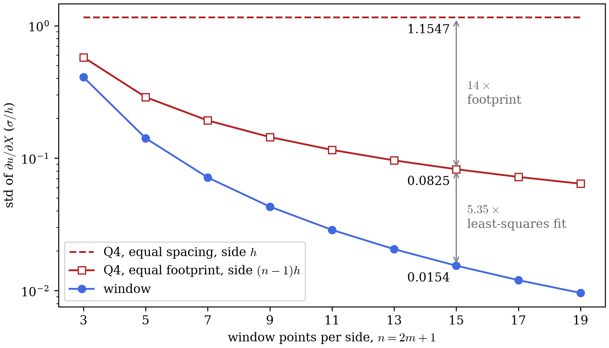
A larger footprint lowers noise and blurs the field. Two methods with the same footprint can still blur by different amounts. Q4 at Equal Resolution checks whether the $5.35\times$ favors the window.

From Gradient to Strain

Fitting $u$ and $v$ gives the four components of the displacement gradient at the window center:

$${\nabla }_0\mathbf{u}=\left[\begin{array}{cc}\partial u/\partial X& \partial u/\partial Y\\ \partial v/\partial X& \partial v/\partial Y\end{array}\right].\text{\hspace{1em}(10.1-16)}$$

The fit uses reference positions $ch$ and $rh$, so this is the Lagrangian gradient. The rest follows Continuum Mechanics:

$$\begin{array}{rl}\mathbf{F}& =\mathbf{I}+{\nabla }_0\mathbf{u},\\ \mathbf{U}& =\sqrt{{\mathbf{F}}^{\top }\mathbf{F}},\\ {\mathbf{E}}^{(0)}& =\ln \mathbf{U}.\end{array}\text{\hspace{1em}(10.1-17)}$$

This page reports the log strain ${\mathbf{E}}^{(0)}$, to match the figures on the pages before it. The fit is linear in the displacements. The strain is not, because $\mathbf{U}$ and $\ln$ are nonlinear. So the noise formulas above hold exactly for ${\nabla }_0\mathbf{u}$. For strain they hold to first order. The 1D Example's Noise showed that log strain noise runs 2% below slope noise at the 2% stretch on these pages.

Fitting the current positions $\mathbf{x}$ instead of $u$ and $v$ gives $\mathbf{F}$ directly as the slope. Both routes agree, because the reference positions $ch$ and $rh$ are exactly linear in $c$ and $r$.

Bias and Resolution

A window reduces variance and blurs the real field. Frequency Response measures that blur on a sine wave. Q4 at Equal Resolution measures a Q4 element's blur on the same wave.

Frequency Response

Take $u=b\sin (kX)$, with wavenumber $k=2\pi /\text{period}$. The wave varies along $X$ only, so every row of the window is identical. The General Window averages its row slopes, so one row's slope gives the window's:

$$\frac{\partial u}{\partial X}{|}_{\text{fit}}=\frac{{\sum }_{c}c{u}_c}{h{\sum }_c{c}^2}.$$

In the continuum limit, the $n$ points become an interval from $-a$ to $a$. Each point stands for a cell $h$ wide, so $a=nh/2$, half the window's extent. With $X=ch$, the sums become integrals:

$$\frac{\partial u}{\partial X}{|}_{\text{fit}}=\frac{{\int }_{-a}^{a}Xb\sin (kX)dX}{{\int }_{-a}^a{X}^{2}dX}=\frac{(2b/k^2)\left(\sin z-z\cos z\right)}{2a^3/3},z=ka.$$

The numerator comes from integration by parts. The true slope at the window center is $bk$. Dividing by it gives the ratio of the fitted slope to the true slope:

$$\begin{array}{rl}T(k)& =\frac{3\left(\sin z-z\cos z\right)}{z^3}\approx 1-\frac{z^2}{10}\text{for }z\ll 1,\\ z& =ka=\frac{knh}{2}.\end{array}\text{\hspace{1em}(10.1-18)}$$

The small-$z$ limit follows from a Taylor expansion, $\sin z-z\cos z\approx z^3/3-z^5/30$. The wave's phase does not change $T$. A wave shifted by $X_0$ splits into $\cos (k{X}_0)\sin (kX)$ plus $\sin (k{X}_0)\cos (kX)$. The $\cos (kX)$ part is even about the center, so the odd weight $X$ integrates it to zero. The fitted slope and the true slope then both scale by $\cos (k{X}_0)$.

$T$ first reaches zero where $\tan z=z$, at $z=4.493$. For $n=15$ and $h=5$ px, $a=37.5$ px, so that zero falls at a period of $2\pi a/4.493=52.4$ px.

Integrating the same numerator by parts for a general $u$ shows what the fit does. Take $\frac{1}{2}(X^2-a^2)$ as the antiderivative of $X$. It vanishes at $X=\pm a$, so the boundary term drops out:

$$\begin{array}{rl}\frac{\partial u}{\partial X}{|}_{\text{fit}}& ={\int }_{-a}^a\varphi (X)\frac{\partial u}{\partial X}dX,\\ \varphi (X)& =\frac{3\left(a^2-X^2\right)}{4a^3}.\end{array}\text{\hspace{1em}(10.1-19)}$$

The weight $\varphi$ is positive and integrates to 1. So the fit averages the true gradient with a parabolic weight. The weight peaks at the center and falls to zero at $X=\pm a$. $T(k)$ is that average applied to the wave's gradient, $bk\cos (kX)$.

The discrete fit skips the continuum limit. It gives $T={\sum }_{c}c\sin (kch)/(kh{\sum }_c{c}^2)$.

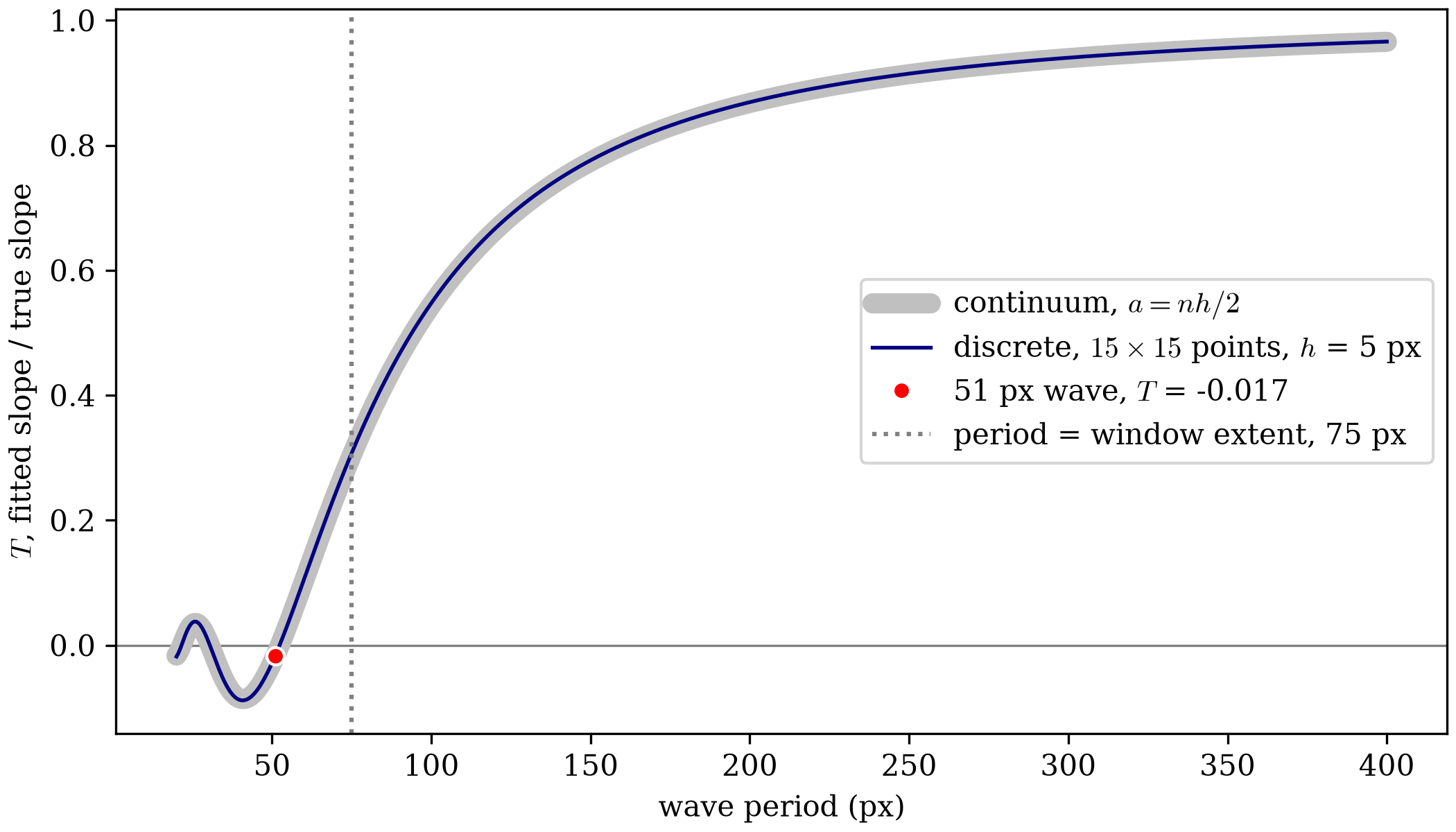
Figure 10.1-11 plots $T$ against the wave period for $n=15$ and $h=5$ px. Kernel Warping found a bias wave in locate_subpixel with a 51 px period:

At a 51 px period, the discrete fit gives $T$ = -0.0167. The continuum formula with $a=nh/2$ gives -0.0173. The discrete $T$ crosses zero at a 52.4 px period. It reaches 0.5 at 94 px and 0.9 at 230 px.

So the window keeps 1.7% of that wave's slope, and reverses its sign. The 51 px period sits 1.4 px below the zero crossing. The 1.7% holds for that period only.

Q4 at Equal Resolution

For the same wave $u=b\sin (kX)$, a Q4 element of side $L$ sees no change in $Y$. So its bottom-edge difference $u_2-u_1$ equals its top-edge difference $u_3-u_4$, and all four Gauss points return the same gradient. Its ratio to the true slope at the element center is

$$T_{\text{Q4}}(k)=\frac{\sin z}{z}\approx 1-\frac{z^2}{6}\text{for }z\ll 1,z=\frac{kL}{2}.\text{\hspace{1em}(10.1-20)}$$

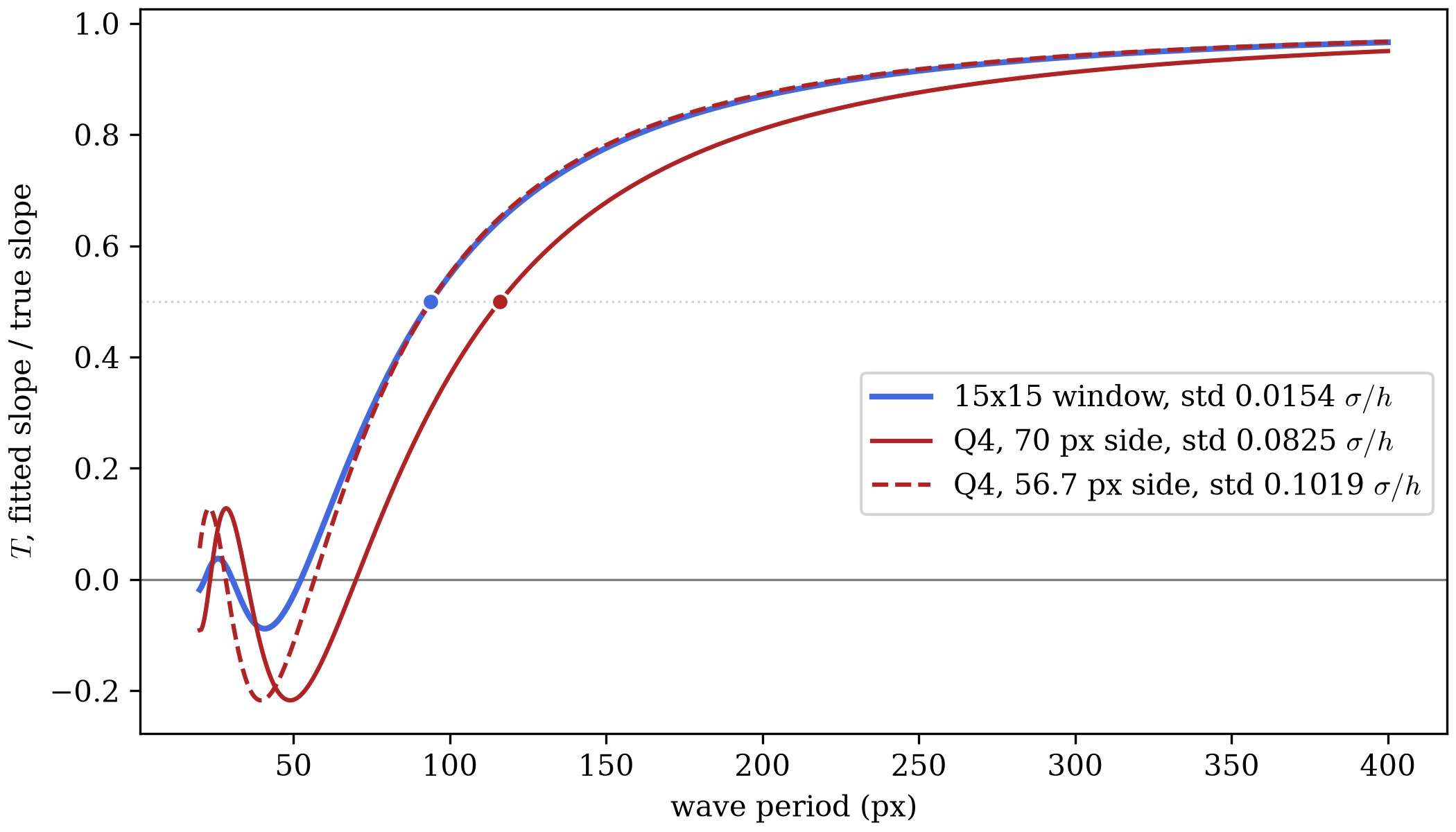
The window's $T$ falls as $1-z^2/10$. At equal footprint, the Q4 element blurs more:

The window keeps half the slope of a 94 px wave. The equal-footprint Q4 element, 70 px on a side, needs a 116 px wave for the same. A Q4 element matches the window's 94 px at 56.7 px on a side. Its standard deviation is then 0.102 $\sigma /h$, 6.6 times the window's 0.0154.

So matching resolution instead of footprint raises the window's lead from $5.35\times$ to $6.6\times$. Equal resolution holds the half-power period fixed at 94 px, so it is the fairer comparison. At equal resolution, the $74.8\times$ equal-spacing lead splits into $11.3\times$ from the footprint and $6.6\times$ from the fit.

Both Q4 elements also pass more of a short wave with its sign reversed. Each one's $T$ bottoms out at $-0.217$, the minimum of $\sin z/z$. The 70 px element reaches it at a 49 px period, and the 56.7 px element at 40 px. The window's $T$ bottoms out at $-0.088$, at a 41 px period. Figure 10.1-12 plots all three responses.

Window Edges

Near the grid boundary, the window truncates. Every tracked point still gets a strain. A truncated window loses the cancellations, so $\sum c$ and $\sum r$ no longer vanish. The matrix is no longer diagonal, and the fit solves the full $3\times 3$ normal equations. Figure 10.1-13 shows interior, edge, and corner windows for $m=3$.

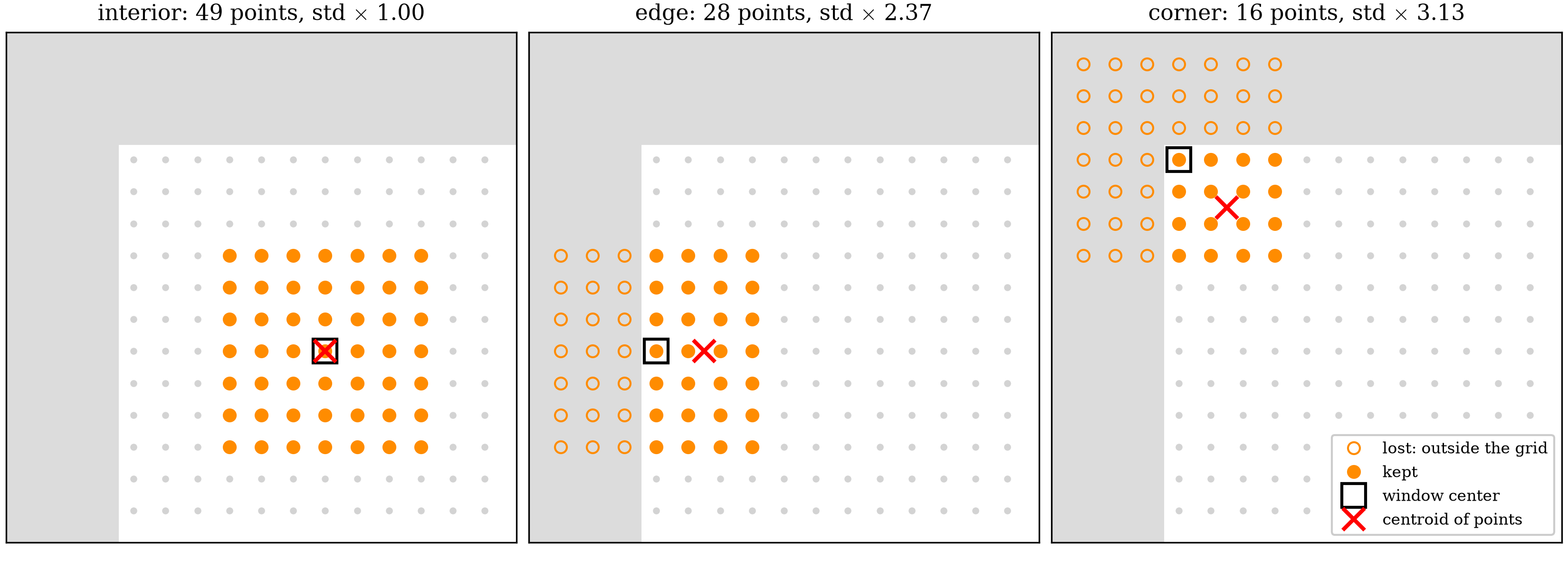
Truncation has two costs. It loses precision, and it moves where the fit measures the gradient. Take the $X$ gradient of a window that lost its $-X$ half, with $m+1$ columns left.

Variance. The slope variance is ${\sigma }^2$ divided by $h^2\sum (c-\bar{c}{)}^2$, where $\bar{c}$ is the mean column of the kept points. That sum falls from $h^{2}n{S}_m$ to $h^{2}nm(m+1)(m+2)/12$. The standard deviation rises by the factor

$$\sqrt{\frac{4(2m+1)}{m+2}}.\text{\hspace{1em}(10.1-21)}$$

At $m=7$, the factor is 2.58. At a corner, the window also keeps only $m+1$ rows. The factor becomes

$$\sqrt{\frac{4(2m+1{)}^2}{(m+1)(m+2)}},\text{\hspace{1em}(10.1-22)}$$

which is 3.54 at $m=7$. At $m=3$, the factors are 2.37 and 3.13, as Figure 10.1-13 shows.

In units of $\sigma /h$, a 15x15 window's standard deviation is 0.0154 in the interior, 0.0398 on an edge, and 0.0545 at a corner. The Q4 element gives 1.155. The edge value is 29 times lower than that. The corner value is 21 times lower.

Location. The fitted slope is a weighted average of the true gradient over the kept points, as Equation 10.1-19 shows. The weights peak at the kept points' centroid and fall to zero at their ends. In a full window, that centroid is the window center. In a truncated window, it sits $mh/2$ inward. At $m=7$ and $h=5$ px, that is 17.5 px. So an edge point reports the strain averaged around a point 17.5 px inside the specimen. If the strain grows by $g$ per pixel toward the edge, the edge value reads $g\cdot mh/2$ too low.

Uniform stretch has $g=0$, so this bias vanishes there. At a hole or a notch, the strain peaks at the edge, so the window underreports the peak.

Overlapping Windows

A window can step by 1 point, so every tracked point gets a strain. Or it can step by $n$ points, so no two windows share a point.

At a step of 1, neighboring windows share $n^2-n$ of their $n^2$ points. For $n=15$, that is 210 of 225. Their errors correlate. The standard deviation across the field then describes the spread of the strain field. It does not describe the uncertainty of independent measurements. Every field spread on this page names its step.

Measured Result

dictk.strain_window.log_strains runs the window on Kernel Warping's tracked positions. The grid has 53x54 points at 5 px spacing. The current image stretches the reference 2% in $X$, so the true $E_{11}$ is $\ln 1.02=19803$ microstrain. The window has $m=7$, so $n=15$. It steps by 1 point. The Q4 row repeats Kernel Warping's baseline on the same positions.

Each of the interior row's 1560 points has a full 15x15 window. Their $E_{11}$ standard deviation is 39 microstrain. Q4 gives 1161 microstrain on the same positions, so the window cuts the spread $30\times$. Over the same interior region, Q4 gives 1181 microstrain, so the $30\times$ holds for matched points too. The interior mean matches $\ln 1.02$ to within 1 microstrain. The Q4 mean sits 48 microstrain above it.

The 39 microstrain leaves out 45.5% of the grid. Those 1302 points sit within 7 points of an edge, so their windows truncate. Their standard deviation is 117 microstrain, 3.0 times the interior value. Their mean sits 73 microstrain below $\ln 1.02$. Over all 2862 points, the standard deviation is 91 microstrain. A full strain field includes its edges, so 91 microstrain is the spread a reader of that field sees.

Strain Field

Figure 10.1-14 redraws Kernel Warping's Q4 field next to the 15x15 window's field. Both panels use the VIC-2D colorbar from Kernel Warping, from 17560 to 22360 microstrain in 16 bands:

Each colorbar band spans 300 microstrain.

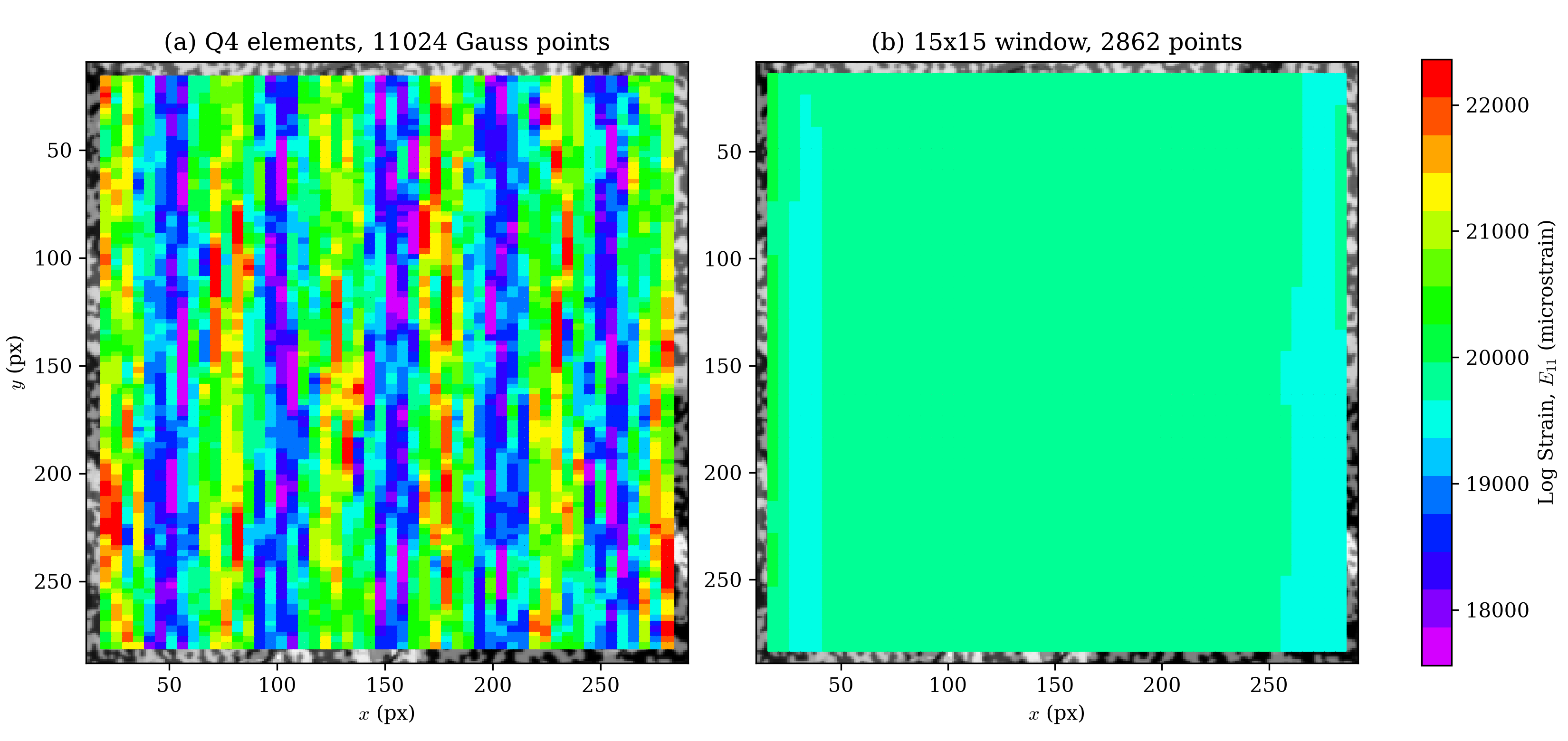
The Q4 field touches all 16 bands, and 2.6% of its Gauss points fall outside the colorbar. The window field touches 3 bands. All 1560 of its interior points fall in one band, from 19660 to 19960 microstrain. The cyan stripes along the left and right sides are truncated columns. Each interior square in panel (b) comes from a fit to 225 tracked positions. Each Q4 Gauss point in panel (a) comes from 4.

Edges and Corners

Window Edges predicts how truncation raises the spread for independent errors. The table tests that prediction on the measured field. It groups the 2862 points by distance to the grid boundary. $d_X$ counts columns to the nearest left or right edge. $d_Y$ counts rows to the nearest top or bottom edge. Both stop at $m=7$, where the window no longer truncates. The table reports the root-mean-square (RMS) error of $E_{11}$ against $\ln 1.02$. The RMS includes bias, and the standard deviation does not. The independent prediction comes from std_factors. The last column gives the largest fraction of a 51 px wave's slope that each window passes, over all phases of the wave.

The column-mean displacement error has an RMS of 0.0076 px. A window fit of it predicts the column-mean $E_{11}$ error with correlation 0.9997.

The independent-error model underpredicts every $X$ edge group. At the edge column, $d_X=0$, the RMS error is 158 microstrain, 4.03 times the interior's 39. The model predicts 2.58. The worst group sits 3 columns in. Its RMS error is 237 microstrain, 6.04 times the interior. The model predicts 1.60 there.

$Y$ edges add 17% to the interior RMS. The top and bottom rows give 46 microstrain, 1.17 times the interior, below the predicted 1.37. The 4 corner points give 187 microstrain, 4.76 times the interior, against a predicted 3.54. The corners also sit at $d_X=0$. Their 187 microstrain sits within 29 microstrain of the $X$ edge's 158.

The tracking error accounts for the gap. Kernel Warping found that the error follows a wave in $X$ with a 51 px period. Panel (a) of Figure 10.1-15 shows the strain error as vertical stripes. It depends on $X$, not on $Y$. Panel (b) averages each column over the 40 rows with a full $Y$ window. The column-mean displacement error has an RMS of 0.0076 px. A window fit of that error predicts the column-mean $E_{11}$ error with correlation 0.9997.

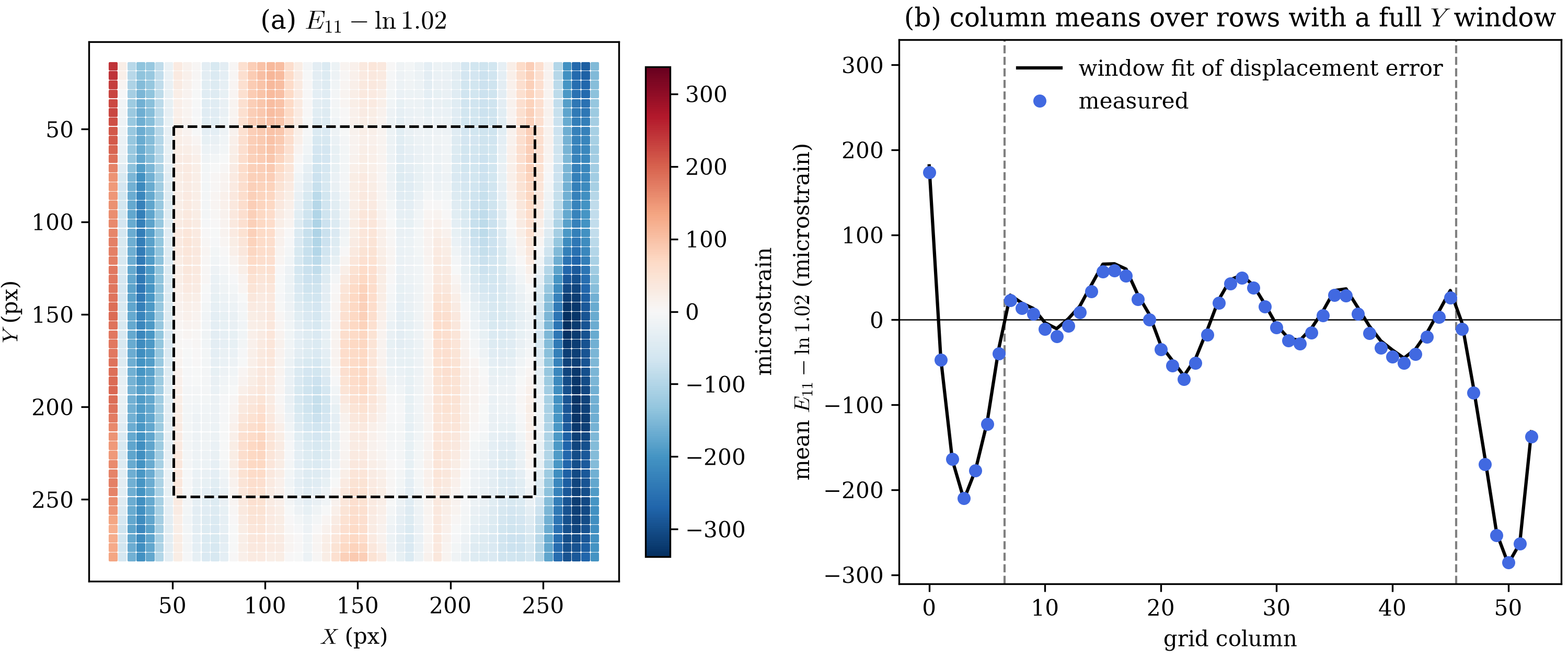
A full window passes 1.7% of the wave's slope. The 51 px period sits 1.4 px from the window's zero crossing at 52.4 px. A truncated window loses that cancellation. At the $X$ edge, it passes up to 52.3%. Three columns in, it passes up to 24.1%. These are upper bounds over the wave's phase. Each $d_X$ group holds only 2 columns, one per side. Its RMS depends on where those 2 columns fall on the wave, so it need not peak at the edge. Here it peaks at $d_X=3$.

The truncated points' 73 microstrain mean offset has the same cause. Their columns sample the wave at phases that do not cancel. Within 5 columns of an $X$ edge, the RMS error runs 2.9 to 6.0 times the interior's. So a field-wide spread from this tracker should report interior and edge points separately.

Window Size

The 15x15 window gives the smallest interior spread of the 9 windows from 3x3 to 19x19. The sweep below reruns the same positions with $m$ from 1 to 9, stepping by 1 point.

The independent-error prediction scales Q4's 1161 microstrain by the window's factor from Noise in a General Window. That scaling sets $\sigma /h$ to $1161/1.1547=1005$ microstrain, so $\sigma =0.0050$ px at $h=5$ px. The tracking error is not independent. Its column-mean wave has an RMS of 0.0076 px, against 0.0029 px row to row. So this $\sigma$ is fitted to Q4's result. It is not a measured independent tracking error.

The measured-error prediction combines two parts in quadrature. The first part fits each window to the column-mean displacement error from Edges and Corners. The second part treats the row-to-row displacement error as independent. That is an approximation. The table's last column is the discrete $T$ of Frequency Response for a 51 px wave.

The row-to-row displacement error has a standard deviation of 0.0029 px.

Figure 10.1-16 plots the table's four spread columns.

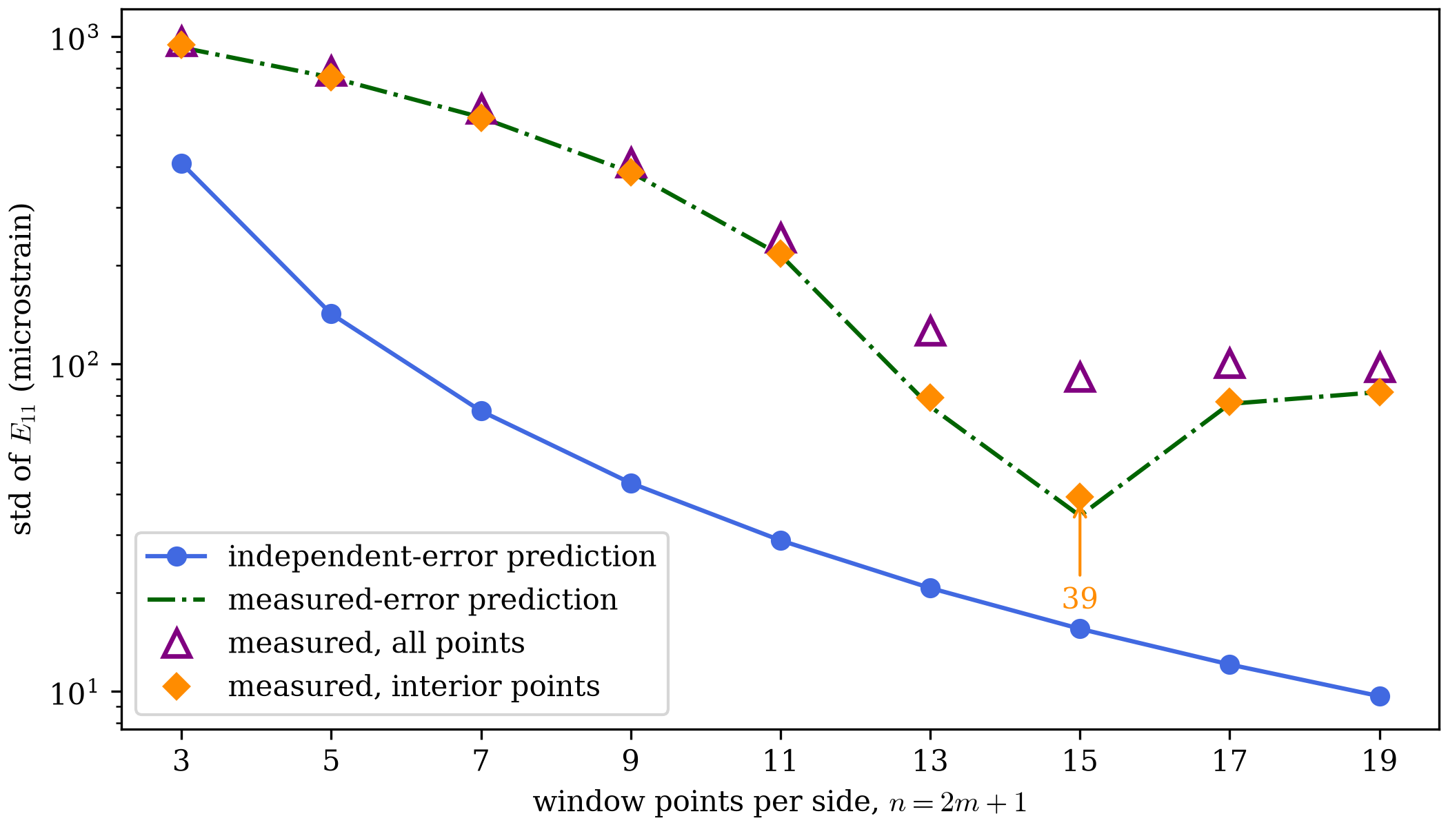
The 39 microstrain is a dip, not a trend. The 13x13 window gives 79 microstrain, and the 17x17 window gives 76. Both are twice the 15x15 value. The 19x19 window gives 82 microstrain, so it averages 1260 points to do worse than 1560 points at $n=15$. The 51 px column shows why. $T$ falls from $+0.089$ at $n=13$ to $-0.017$ at $n=15$, and then to $-0.074$ at $n=17$. The window passes the least of the wave's slope at $n=15$, and that wave dominates the error.

The independent-error prediction misses that shape. It falls at every step, from 410 microstrain at $n=3$ to 9.7 at $n=19$. The measured spread sits 2.3 times above it at $n=3$, 2.5 times at $n=15$, and 8.5 times at $n=19$. The measured-error prediction stays within 19 microstrain of the measured spread at $n=3$, and within 5 microstrain from $n=5$ to 19.

The all-points spread also bottoms out at $n=15$, at 91 microstrain. Its minimum is shallower. The 17x17 and 19x19 windows give 101 and 98 microstrain, because those windows truncate at 1456 and 1602 of the 2862 points.

The best window size depends on the error's period. This tracker's error follows a 51 px wave, and a 15x15 window at 5 px spacing happens to land 1.4 px from that wave's zero crossing. A tracker or image with a different error period would move the dip. Choosing $n$ needs a sweep like this one, on data with a known answer.

Continue to Discontinuities.