Simple Shear

Note: The source code for this section is listed below.

In this section, we cover simple shear, a deformation that illustrates several concepts without being too complicated. That said, we will find that simple shear isn't quite as trivial as its name would suggest. In fact, a paper titled Simple shear is not so simple¹ reviews some details not discussed here.

Figure 2.2-1 illustrates simple shear, with relative motion of planes normal to the vertical axis. For all configurations (reference and current):

• Horizontal fibers remain horizontal.
• The length of horizontal fibers remains constant.
• The vertical distance between the horizontal fibers remains constant.
• The body's volume is constant. The deformation is isochoric since $\det (\mathbf{F})=1$.

The relative motion is characterized by the non-dimensional ratio of length $a$ per unit height, where $a\in \mathbb{R}\subset [0,\infty )$. The angle, $\gamma \in \mathbb{R}\subset [0,\pi /2)$, subtended by simple shear is $\gamma =\arctan (a)$. In the limit as $a\mapsto \infty$, the shear angle $\gamma \mapsto \pi /2$. For small values of $a$, the small-angle assumption is valid, with $\tan (\gamma )\approx \gamma \approx a$.

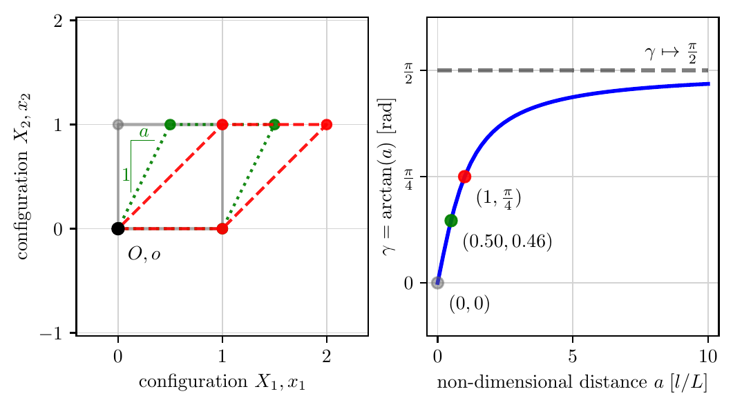
Source: simple_shear.py

Rate-Independent Form

The simple shear deformation $\mathbf{\phi }$ in rate-independent form is

$$\mathbf{\phi }(\mathbf{X})=(X_1+a{X}_2){\mathbf{e}}_1+X_2{\mathbf{e}}_2+X_3{\mathbf{e}}_3.$$

The deformation gradient $\mathbf{F}$ is

$$\begin{array}{rl}\mathbf{F}& :={\mathbf{e}}_i\frac{\partial {\phi }_i}{\partial X_J}{\mathbf{E}}_J={\mathbf{e}}_1\otimes {\mathbf{E}}_1+a{\mathbf{e}}_1\otimes {\mathbf{E}}_2+{\mathbf{e}}_2\otimes {\mathbf{E}}_2+{\mathbf{e}}_3\otimes {\mathbf{E}}_3\\ & =\{{\mathbf{e}}_1{\mathbf{e}}_2{\mathbf{e}}_3\}\left[\begin{array}{ccc}1& a& 0\\ 0& 1& 0\\ 0& 0& 1\end{array}\right]\left\{\begin{array}{c}{\mathbf{E}}_1\\ {\mathbf{E}}_2\\ {\mathbf{E}}_3\end{array}\right\}⟺{\mathbf{F}}_{iJ}=\left[\begin{array}{ccc}1& a& 0\\ 0& 1& 0\\ 0& 0& 1\end{array}\right].\end{array}$$

Note that the volume remains constant for all deformations since $\det (\mathbf{F})=1$. The deformation thus belongs to the group of isochoric motions. The right Cauchy-Green strain, $\mathbf{C}:={\mathbf{F}}^T\mathbf{F}$, in simple shear, is

$$\begin{array}{rl}\mathbf{C}=& {\mathbf{E}}_1\otimes {\mathbf{E}}_1+a({\mathbf{E}}_1\otimes {\mathbf{E}}_2+{\mathbf{E}}_2\otimes {\mathbf{E}}_1)+\\ & (a^2+1){\mathbf{E}}_2\otimes {\mathbf{E}}_2+{\mathbf{E}}_3\otimes {\mathbf{E}}_3⟺{\mathbf{C}}_{IJ}=\left[\begin{array}{ccc}1& a& 0\\ a& a^2+1& 0\\ 0& 0& 1\end{array}\right].\end{array}$$

The principal directions of $\mathbf{C}$ are given with the three eigenvectors $\{{\mathbf{N}}_1,{\mathbf{N}}_2,{\mathbf{N}}_3\}$ and their respective eigenvalues ${\lambda }_1^2,{\lambda }_2^2,{\lambda }_3^2$,

$$\mathbf{C}=\sum _{\alpha =1}^3{\lambda }_{\alpha }^2{\mathbf{N}}_{\alpha }\otimes {\mathbf{N}}_{\alpha }.$$

For simple shear, the eigenvalues of $\mathbf{C}$ and their corresponding eigenvectors, satisfying $[\mathbf{C}]\{\mathbf{N}\}={\lambda }^2\{\mathbf{N}\}$, are

$$\begin{array}{rl}{\lambda }_1^2=\frac{1}{2}\left(a^2+a\sqrt{a^2+4}+2\right),& \text{and}{\mathbf{N}}_1={\left\{\frac{1}{2}\left(-a+\sqrt{a^2+4}\right),1,0\right\}}^T;\\ {\lambda }_2^2=1,& \text{and}{\mathbf{N}}_2=\{0,0,1{\}}^T;\\ {\lambda }_3^2=\frac{1}{2}\left(a^2-a\sqrt{a^2+4}+2\right),& \text{and}{\mathbf{N}}_3={\left\{\frac{1}{2}\left(-a-\sqrt{a^2+4}\right),1,0\right\}}^T.\end{array}$$

The Green-Lagrange strain, $\mathbf{E}:=\frac{1}{2}(\mathbf{C}-\mathbf{I})$, in simple shear is

$${\mathbf{E}}_{IJ}=\frac{1}{2}\left[\begin{array}{ccc}0& a& 0\\ a& a^2& 0\\ 0& 0& 0\end{array}\right].$$

The left Cauchy-Green strain, $\mathbf{b}:=\mathbf{F}{\mathbf{F}}^T$, (and its inverse), in simple shear, are

$${\mathbf{b}}_{ij}=\left[\begin{array}{ccc}{a}^2+1& a& 0\\ a& 1& 0\\ 0& 0& 1\end{array}\right],\text{and}{\mathbf{b}}_{ji}^{-1}=\left[\begin{array}{ccc}1& -a& 0\\ -a& a^2+1& 0\\ 0& 0& 1\end{array}\right].$$

The Almansi-Euler strain, $\mathbf{e}:=\frac{1}{2}(\mathbf{I}-{\mathbf{b}}^{-1})$, for simple shear is

$${\mathbf{e}}_{ij}=\frac{1}{2}\left[\begin{array}{ccc}0& a& 0\\ a& -a^2& 0\\ 0& 0& 0\end{array}\right].$$

Source

simple_shear.py

"""Demonstrate simple shear deformation of a square body."""

from typing import Tuple
import os
import numpy as np
from numpy.typing import NDArray

from matplotlib import rc
import matplotlib.pyplot as plt
from matplotlib.ticker import MultipleLocator

rc("text", usetex=True)
# rc('font', **{'family': 'serif', 'serif': ['Computer Modern Roman']})
rc("font", family="serif")


def rotate(x0: NDArray, y0: NDArray, rotation: float) -> Tuple[NDArray, NDArray]:
    """Given list of reference points (x0, y0), rotate them about the
    z-axis by rotation angle (radians) to the current points (x1, y1).
    """
    x1 = np.cos(rotation) * x0 - np.sin(rotation) * y0
    y1 = np.sin(rotation) * x0 + np.cos(rotation) * y0
    return x1, y1


def simple_shear(x0: NDArray, y0: NDArray, shear: float) -> Tuple[NDArray, NDArray]:
    """Given a list of reference points (x0, y0), simple shear them in
    the x-axis by distance shear_x (Length) to the current points (x1, y1).
    """
    x1 = x0 + shear * y0
    y1 = y0
    return x1, y1


def draw_shape(
    axis,
    xs: np.ndarray,
    ys: np.ndarray,
    color: str = "dimgray",
    linestyle: str = "-",
    alpha: float = 1.0,
):
    """Draw the body and points."""

    # Draw body outline
    axis.plot(
        xs,
        ys,
        color=color,
        linestyle=linestyle,
        alpha=alpha,
    )  # body outline

    # Plot points on the body
    axis.plot(xs, ys, "o", color=color, markersize=5, alpha=alpha)


SHOW = False
SAVE = True

fig = plt.figure(figsize=(6, 3))  # inches, (wide, tall)
ax1 = fig.add_subplot(1, 2, 1)
ax2 = fig.add_subplot(1, 2, 2)

# Subfigure 1

OFFSET_X = 0
OFFSET_Y = 0
RADTODEG = 180.0 / np.pi
DEGTORAD = 1.0 / RADTODEG

# Defined reference configuration path, in a closed circle
xs_0 = np.array([0, 1, 1, 0, 0])
ys_0 = np.array([0, 0, 1, 1, 0])

# Draw reference shape
draw_shape(axis=ax1, xs=xs_0, ys=ys_0, color="dimgray", linestyle="-", alpha=0.5)

# Draw first sheared shape
SHEAR_1 = 0.5
(xs_1, ys_1) = simple_shear(xs_0, ys_0, shear=SHEAR_1)
draw_shape(axis=ax1, xs=xs_1, ys=ys_1, color="green", linestyle=":", alpha=0.9)

# Draw second sheared shape
SHEAR_2 = 1.0
(xs_2, ys_2) = simple_shear(xs_0, ys_0, shear=SHEAR_2)
draw_shape(axis=ax1, xs=xs_2, ys=ys_2, color="red", linestyle="--", alpha=0.9)

# Draw origin point
ax1.plot(0, 0, "o", color="black", label="origin = (0, 0, 0)")
# Draw origin label
ax1.text(0.25, -0.25, r"$O, o$", ha="center", va="center")

# Draw 1:a rise over run lines
SCALE = 0.90  # scale
HAIRLINE_OFFSET_Y = 0.1
epsx, epsy = 0.125, 0.25 + HAIRLINE_OFFSET_Y
slope_x, slope_y = np.array([0, 0, 0.25]) * SCALE, np.array([0, 0.5, 0.5])
ax1.plot(slope_x + epsx, slope_y + epsy, lw=0.5, color="green")
ax1.text(0.125, 0.5, "1", color="green", ha="right", va="center")
ax1.text(0.25, 0.88, r"$a$", color="green", ha="center")


# SHEAR_12 = 0.5  # Length units, shear in the X_1 direction
# draw(ax1, ux=OFFSET_Y, uy=OFFSET_Y, ur=dr, shear=SHEAR_12, t0=False, c="green", ls=":")

# SHEAR_12 = 1.0  # Length units, shear in the X_1 direction, larger shear
# draw(ax1, ux=OFFSET_X, uy=OFFSET_X, ur=dr, shear=SHEAR_12, t0=False, c="red", ls="--")


ax1.axis("equal")
# ax2.axis('equal')
# major axes
ax1.xaxis.set_major_locator(MultipleLocator(1.0))
ax1.yaxis.set_major_locator(MultipleLocator(1.0))
ax2.xaxis.set_major_locator(MultipleLocator(1.0))
ax2.yaxis.set_major_locator(MultipleLocator(1.0))
# minor axes
# ax1.xaxis.set_minor_locator(MultipleLocator(0.5))
# ax1.yaxis.set_minor_locator(MultipleLocator(0.5))

ax1.grid(
    visible=True, which="major", linestyle="solid", linewidth=0.5, color="lightgray"
)  # FIX APPLIED HERE
ax2.grid(
    visible=True, which="major", linestyle="solid", linewidth=0.5, color="lightgray"
)  # FIX APPLIED HERE
#
# ax.grid(b=True, which='minor', linestyle=':')
ax1.set_xlabel(r"configuration $X_1, x_1$")
ax1.set_ylabel(r"configuration $X_2, x_2$")

# Subfigure 2

X_MIN = 0
X_MAX = 10
epsx, epsy = 0.4, np.pi / 16
x = np.linspace(X_MIN, X_MAX)
y = np.arctan(x)
ax2.plot(x, y, linewidth=2, color="blue")
ax2.text(
    X_MAX - epsx,
    np.pi / 2 + epsy / 2,
    r"$\gamma \mapsto \frac{\pi}{2}$",
    ha="right",
    backgroundcolor="white",
)
ax2.plot(
    [X_MIN, X_MAX],
    np.pi / 2 * np.array([1, 1]),
    lw=2,
    alpha=0.5,
    color="black",
    linestyle="--",
    zorder=4,
)

ax2.plot(0, 0, "o", color="dimgray", alpha=0.5, zorder=4)
ax2.text(0 + epsx, 0 - epsy, r"$(0, 0)$", backgroundcolor="white")

ax2.plot(0.5, 0.46, "o", color="green", alpha=0.9, zorder=4)
ax2.text(0.50 + epsx, 0.46 - epsy, r"$(0.50, 0.46)$", backgroundcolor="white")

ax2.plot(1, np.pi / 4, "o", color="red", alpha=0.9, zorder=4)
ax2.text(1 + epsx, np.pi / 4 - epsy, r"$(1, \frac{\pi}{4})$", backgroundcolor="white")

ax2.set_xlabel(r"non-dimensional distance $a\;[l/L]$")
ax2.set_ylabel(r"$\gamma = \arctan(a)$ [rad]")
# https://matplotlib.org/3.1.1/gallery/ticks_and_spines/tick-locators.html
# ax2.xaxis.set_major_locator(ticker.FixedLocator([0, 5, 10]))
ax2.set_xticks([0, 5, 10])
ax2.set_yticks([0, np.pi / 4, np.pi / 2])
ax2.set_yticklabels(["0", r"$\frac{\pi}{4}$", r"$\frac{\pi}{2}$"])

ax1.set_xlim(-epsx, 2 + epsx)
ax2.set_xlim(0 - epsx, X_MAX + epsx)
eps = np.pi / 8
ax2.set_ylim(0 * np.pi / 4 - eps, np.pi / 2 + eps)

if SHOW:
    plt.show()

if SAVE:
    script_name = os.path.basename(__file__)
    figure_name = os.path.splitext(script_name)[0]
    print(f"Saving figure as {figure_name}.pdf")
    fig.savefig(figure_name + ".pdf", bbox_inches="tight")

References

1. Destrade M, Murphy JG, Saccomandi G. Simple shear is not so simple. International Journal of Non-Linear Mechanics. 2012 Mar 1;47(2):210-4. download ↩