Parallelization
Multi-Point Motion just ran 12
independent calls to
dictk.translation.locate — one
per point, each doing its own FFT-based phase correlation — to verify
every point's displacement. We anticipate the need to process a very
large number of point-to-point correspondences to support large-scale
DIC work — a real finite element mesh (see Finite Element
Method) can easily have thousands-to-millions
of nodes, not the 12 points in the simple grid above. Each point
correspondence is independent of every other: locating point never
reads or writes anything locating point touches. That independence
isn't just a convenient property to point out —
dictk.grid.locate is already written to
exploit it. Its entire body is a single map over reference_points, one
call to dictk.translation.locate
per point, accumulating no shared state between iterations:
return [
    translation.locate(
        reference_image=reference_image,
        current_image=current_image,
        reference_point=reference_point,
        search_center=search_center,
        kernel_margin_width=kernel_margin_width,
        kernel_margin_height=kernel_margin_height,
        search_margin_width=search_margin_width,
        search_margin_height=search_margin_height,
    )
    for reference_point, search_center in zip(reference_points, search_centers)
]
Because every iteration is already independent, parallelizing it is a
matter of swapping this list comprehension for a parallel map over the
same per-point calls. It is not a redesign.
dictk.grid.locate does exactly that
today, behind two extra keyword-only parameters: max_workers and
executor. Default max_workers=None stays sequential, the loop above,
byte-identical to locate's original behavior. A positive integer
switches to a worker pool instead.
Which pool, though, is not obvious. It needs its own explanation first.
Threads, Processes, and the GIL
CPython has a Global Interpreter Lock (GIL): only one thread can
execute Python bytecode at a time, even on a machine with many cores. A
plain Python for loop split across threads would not run any faster.
Each thread would still wait its turn for the same lock.
C extensions can release the GIL during their own C-level computation,
though. NumPy and SciPy both do this for many operations. The FFT
dictk.translation.locate actually runs is one of them —
skimage.registration.phase_cross_correlation calls scipy.fft.fftn
and scipy.fft.ifftn internally, not the Python-level fallback, and
scipy.fft releases the GIL for the duration of its own C computation.
So threads can run FFT correlations in true parallel. The GIL is not
held the whole time.
Whether that helps depends on scale. A tiny FFT finishes almost instantly. Most of the wall-clock time around it is Python-level overhead: function calls, object construction, array slicing. Releasing the GIL for a few microseconds does not buy much when the thread scheduling and GIL reacquisition around it cost microseconds too. A large FFT is different. Once the C computation itself dominates the call, the GIL-released fraction of wall-clock time dominates too, and threads start to pay off.
Threads vs. Processes: Two Different Costs
A ThreadPoolExecutor shares the caller's own memory. No pickling, no
process spawn. Cheap to start. But every task still pays a GIL
scheduling cost, and that cost does not shrink as task count grows. Run
one task or a million, each one pays it individually.
A ProcessPoolExecutor is different. Each worker is a separate OS
process, with its own interpreter and its own GIL. It gets true
parallelism regardless of whether the target function releases the GIL
at all. The cost moves elsewhere: data has to be pickled across the
process boundary, and on macOS (which spawns fresh interpreters rather
than forking) each worker re-imports NumPy, SciPy, and scikit-image
from scratch before it can do any work. That cost is mostly fixed and
paid once, when the pool starts.
That is the real asymmetry: processes pay once, threads pay every time. More tasks amortize a process pool's fixed startup cost. More tasks do not shrink a thread pool's per-task cost. Which one wins depends on both how big each task is and how many tasks there are — not on either alone.
Measuring the Trade Space
Rather than guess, measure.
parallelization_bench.py (full source
below) times sequential, threaded, and process-pool execution of
phase_cross_correlation across three scenarios. Correlation size and
point count are not independent in a real DIC problem — a
million-point mesh only makes sense with a small subset per point — so
this is three targeted scenarios, not one brute-force grid:
book_scale: this book's own kernel/search size (40 pixels), point count climbing from 100 to 1,000,000. Does point count alone ever create a crossover, at a size this small?large_subset: only 16 points, correlation size climbing from 200 to 2,000 pixels. Where does the threads crossover sit, as a function of size alone?realistic_mesh: a closer match to an actual finite element mesh — moderate correlation size (100 or 200 pixels), point count climbing from 1,000 to 100,000.
This sweep takes several minutes to run (the book_scale scenario's
1,000,000-point case alone runs over a minute) — far too slow to
re-run on every build the way this book's other figures do. Its results
are measured once and committed alongside the script that produced
them, not regenerated live. The table below still reads live from that
committed data, so it always matches the file on disk:
| Scenario | Size | Points | Sequential (s) | Threads (s) | Threads speedup | Processes (s) | Processes speedup |
|---|---|---|---|---|---|---|---|
| book_scale | 40 | 100 | 0.00752 | 0.02057 | 0.366x | 0.77663 | 0.01x |
| book_scale | 40 | 1000 | 0.07277 | 0.18621 | 0.391x | 0.99653 | 0.073x |
| book_scale | 40 | 10000 | 0.70866 | 1.83165 | 0.387x | 2.06538 | 0.343x |
| book_scale | 40 | 100000 | 7.16526 | 18.32857 | 0.391x | 14.26206 | 0.502x |
| book_scale | 40 | 1000000 | 71.65412 | 169.90165 | 0.422x | 116.62403 | 0.614x |
| large_subset | 200 | 16 | 0.01608 | 0.0087 | 1.847x | 0.83688 | 0.019x |
| large_subset | 500 | 16 | 0.10876 | 0.02691 | 4.041x | 0.82919 | 0.131x |
| large_subset | 1000 | 16 | 0.46973 | 0.10719 | 4.382x | 0.99717 | 0.471x |
| large_subset | 2000 | 16 | 2.2572 | 0.50896 | 4.435x | 2.85197 | 0.791x |
| realistic_mesh | 100 | 1000 | 0.26763 | 0.24035 | 1.114x | 0.8058 | 0.332x |
| realistic_mesh | 100 | 10000 | 2.6885 | 2.45357 | 1.096x | 2.13847 | 1.257x |
| realistic_mesh | 100 | 100000 | 26.81134 | 24.32667 | 1.102x | 15.24042 | 1.759x |
| realistic_mesh | 200 | 1000 | 0.95522 | 0.34662 | 2.756x | 1.02504 | 0.932x |
| realistic_mesh | 200 | 10000 | 9.59174 | 3.43856 | 2.789x | 4.41874 | 2.171x |
| realistic_mesh | 200 | 100000 | 98.60379 | 31.72111 | 3.108x | 36.23009 | 2.722x |
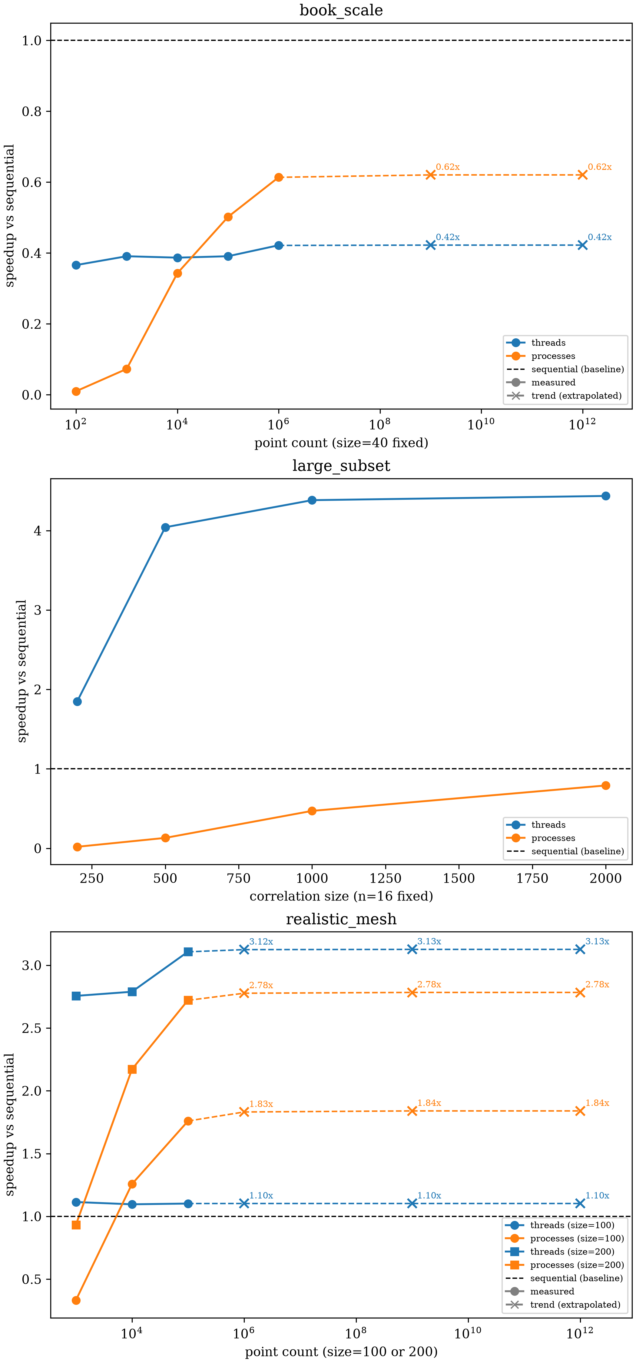
spawn start method). Solid lines are measured data. Dashed lines are trend extrapolations — a straight-line time-vs-point-count fit, projected out to 106, 109, and 1012 points. Top: at this book's own 40-pixel scale, sequential wins at every point count tested, up to 1,000,000, and the trend predicts it keeps winning — processes plateau near 0.62x, threads near 0.42x, even out to a trillion points. Middle: at only 16 points, threads win decisively once correlations are large enough; processes never recover their fixed startup cost. Not extrapolated: this panel's x-axis is correlation size, not point count, and a subset a billion pixels wide isn't physical. Bottom: with enough points, both help, and processes close the gap on threads as point count grows; the trend predicts each pair levels off close to its last measured value.Four findings, read directly off that data:
- At this book's own scale, sequential always wins. 1,000,000 points at 40 pixels still favors sequential (71.7s) over both threads (169.9s) and processes (116.6s). Point count alone never creates a crossover at this size — not at 100 points, not at a million.
- Few points, large correlations: threads win, processes cannot recover. At 2,000 pixels with only 16 points, threads reach 4.4x. Processes reach only 0.79x — still slower than sequential. Sixteen tasks is not enough to amortize a process pool's fixed startup cost, no matter how large each individual task is.
- Many points, moderate correlations: processes catch up, and can pass threads. At 100 pixels, processes start behind threads (0.33x vs. 1.11x at 1,000 points) but overtake them by 100,000 points (1.76x vs. 1.10x). More tasks keep amortizing a process pool's fixed cost long after a thread pool's per-task cost has stopped improving.
- The trend, extrapolated to Path Forward's north-star scale,
predicts a plateau, not a crossover. Fitting a straight line to
each method's measured time-vs-point-count and reading off the
resulting speedup ratio at 106, 109, and
1012 points:
book_scale's ordering never flips (processes settle near 0.62x, threads near 0.42x, both still slower than sequential);realistic_mesh's pairs settle close to their last measured value (size=100: threads 1.10x, processes 1.84x; size=200: threads 3.13x, processes 2.78x). This is a linear extrapolation from a handful of measured points, not a new measurement — a hypothesis worth testing at real scale, not a settled result.
Using max_workers
dictk.grid.locate accepts max_workers and executor directly now,
no sketch required. Run it against the same 12-point grid Multi-Point
Motion already tracked,
sequential and concurrent side by side:
from dictk.grid import Executor, locate

sequential = locate(
    reference_image=reference_image,
    current_image=current_image,
    reference_points=points,
    kernel_margin_width=20,
    kernel_margin_height=20,
    search_margin_width=48,
    search_margin_height=52,
)
threaded = locate(
    reference_image=reference_image,
    current_image=current_image,
    reference_points=points,
    kernel_margin_width=20,
    kernel_margin_height=20,
    search_margin_width=48,
    search_margin_height=52,
    max_workers=4,
    executor=Executor.THREAD,
)
print(f"results match: {sequential == threaded}")
results match: True
The results match, as they must — max_workers changes how the 12
points are tracked, not what answer each one finds. It does not change
the runtime in any way worth showing here, either. Twelve points at 40
pixels is deep in the book_scale regime above: sequential wins.
Demonstrating correctness at this scale, not speed, is the honest thing
to show.
Choosing an Executor
Given the measured trade space, not a guess:
- This book's own examples (small kernels, small search areas):
don't parallelize at all. Leave
max_workers=None. Sequential wins here regardless of point count. - Few points, each with a large correlation:
Executor.THREAD. Processes cannot recover their fixed cost across only a handful of tasks, no matter how large each one is. - Many points, each with a moderate-to-large correlation (the
closest match to a real finite element mesh): either pool helps;
Executor.PROCESScloses the gap on threads as point count grows, and can pass it. - Unsure which regime a problem falls in?
Executor.THREADislocate's default for exactly this reason. It is never catastrophically worse than sequential, unlike a process pool at low point counts, even though it is not always the fastest option available.
parallelization_bench.py
"""Benchmark: sequential vs. threads vs. processes for
skimage.registration.phase_cross_correlation, at varying correlation
sizes and call counts.

Not part of the dictk package -- a standalone, one-time measurement
script, matching the convention simple_shear.py already sets. Its
output (parallelization_bench.csv, parallelization_bench.png) is
committed alongside it rather than regenerated on every book build: the
full sweep takes several minutes (the 1,000,000-call case alone runs
over a minute), far too slow for the live cmdrun re-execution every
other figure in this book uses. Parallelization.md prints this script's
full source inline (see its own "parallelization_bench.py" section) so
the numbers stay checkable even though they are not live.

Must be a real module, not `python3 -c` -- ProcessPoolExecutor needs a
real, importable, top-level function to hand to spawned workers, the
same constraint dictk.grid._locate_worker exists for.

Re-run with: python3 parallelization_bench.py
"""

import csv
import os
import time
from concurrent.futures import ProcessPoolExecutor, ThreadPoolExecutor

import matplotlib.pyplot as plt
import numpy as np
from skimage.registration import phase_cross_correlation

WORKERS = os.cpu_count()

CSV_PATH = "parallelization_bench.csv"
FIGURE_PATH = "parallelization_bench.png"

# Point count and correlation size are not independent in a real DIC
# problem -- a million-point mesh only makes sense with small subsets
# per point. Three scenarios instead of one brute-force grid, each
# answering a different question:
SCENARIOS = {
    # This book's own teaching scale (kernel/search sizes throughout
    # Single/Multi-Point Motion). Does point count alone ever create a
    # crossover, at a size this small?
    "book_scale": [(40, n) for n in [100, 1_000, 10_000, 100_000, 1_000_000]],
    # Few points, growing correlation size. Where does the threads
    # crossover actually sit, as a function of size alone?
    "large_subset": [(size, 16) for size in [200, 500, 1000, 2000]],
    # A more realistic finite element mesh: moderate subset size,
    # climbing point count. Does the processes-vs-threads balance shift
    # as point count grows?
    "realistic_mesh": [(100, n) for n in [1_000, 10_000, 100_000]]
    + [(200, n) for n in [1_000, 10_000, 100_000]],
}


def one(args: tuple[np.ndarray, np.ndarray]):
    """One correlation. Module-level and single-positional-argument on
    purpose -- see the module docstring."""
    kernel, search = args
    return phase_cross_correlation(kernel, search, normalization="phase")


def make_args(size: int, n_calls: int, seed: int = 42):
    """`n_calls` copies of the same random kernel/search pair at `size`.

    The same pair repeated, not `n_calls` distinct random pairs: this
    benchmark measures call overhead, not correlation accuracy, so
    identical inputs keep every call's own work identical too."""
    rng = np.random.default_rng(seed)
    kernel = rng.random((size, size))
    search = rng.random((size, size))
    return [(kernel, search)] * n_calls


def time_sequential(args) -> float:
    t0 = time.perf_counter()
    for x in args:
        one(x)
    return time.perf_counter() - t0


def time_threads(args) -> float:
    t0 = time.perf_counter()
    with ThreadPoolExecutor(max_workers=WORKERS) as pool:
        list(pool.map(one, args))
    return time.perf_counter() - t0


def time_processes(args) -> float:
    t0 = time.perf_counter()
    with ProcessPoolExecutor(max_workers=WORKERS) as pool:
        list(pool.map(one, args))
    return time.perf_counter() - t0


def run_case(scenario: str, size: int, n_calls: int, writer: csv.DictWriter) -> None:
    args = make_args(size, n_calls)

    sequential_s = time_sequential(args)
    threads_s = time_threads(args)
    processes_s = time_processes(args)

    writer.writerow(
        {
            "scenario": scenario,
            "size": size,
            "n_calls": n_calls,
            "workers": WORKERS,
            "sequential_s": round(sequential_s, 5),
            "threads_s": round(threads_s, 5),
            "processes_s": round(processes_s, 5),
            "threads_speedup": round(sequential_s / threads_s, 3),
            "processes_speedup": round(sequential_s / processes_s, 3),
        }
    )
    print(
        f"[{scenario}] size={size:5d} n={n_calls:8d}  "
        f"sequential={sequential_s:8.3f}s  "
        f"threads={threads_s:8.3f}s (x{sequential_s / threads_s:5.2f})  "
        f"processes={processes_s:8.3f}s (x{sequential_s / processes_s:5.2f})",
        flush=True,
    )


def run_sweep() -> None:
    fieldnames = [
        "scenario",
        "size",
        "n_calls",
        "workers",
        "sequential_s",
        "threads_s",
        "processes_s",
        "threads_speedup",
        "processes_speedup",
    ]
    with open(CSV_PATH, "w", newline="") as f:
        writer = csv.DictWriter(f, fieldnames=fieldnames)
        writer.writeheader()
        for scenario, cases in SCENARIOS.items():
            for size, n_calls in cases:
                run_case(scenario, size, n_calls, writer)
                f.flush()
    print(f"\nWrote {CSV_PATH}")


# Point counts to extrapolate speedup trends out to, tying directly to
# the "north star" scale in Path Forward (billions of correlations,
# staying under a trillion by design). Only scenarios whose x-axis is
# point count (book_scale, realistic_mesh) get this treatment --
# large_subset's x-axis is correlation *size*, and extrapolating a
# subset's side length out to a billion pixels isn't physical.
EXTRAPOLATION_TARGETS = [1_000_000, 1_000_000_000, 1_000_000_000_000]


def _trend_line(ns, seq_times, other_times, targets):
    """Fit a linear time-vs-n trend (time = a*n + b) to `seq_times` and
    `other_times` independently, then extrapolate the *speedup ratio*
    (their fitted-time ratio) out to every target beyond the last real
    data point.

    Returns `(xs, speedups, marks)`: `xs`/`speedups` start at the last
    *measured* point (so a plotted dashed line picks up exactly where
    the solid measured line ends, no visual gap) and run through every
    target; `marks` is just the subset of targets genuinely beyond the
    measured range, for placing "predicted value" markers.
    """
    a_seq, b_seq = np.polyfit(ns, seq_times, 1)
    a_other, b_other = np.polyfit(ns, other_times, 1)
    last_n = ns[-1]
    marks = [t for t in targets if t > last_n]
    xs = [last_n] + marks
    speedups = [(a_seq * n + b_seq) / (a_other * n + b_other) for n in xs]
    return xs, speedups, marks


def _add_trend(ax, ns, seq_times, other_times, color):
    xs, speedups, marks = _trend_line(ns, seq_times, other_times, EXTRAPOLATION_TARGETS)
    ax.plot(xs, speedups, linestyle="--", color=color, linewidth=1.2)
    mark_speedups = speedups[-len(marks) :] if marks else []
    ax.plot(
        marks,
        mark_speedups,
        linestyle="none",
        marker="x",
        color=color,
        markersize=7,
        markeredgewidth=1.5,
    )
    for n, s in zip(marks, mark_speedups):
        ax.annotate(
            f"{s:.2f}x",
            (n, s),
            textcoords="offset points",
            xytext=(4, 4),
            fontsize=7,
            color=color,
        )


def plot_summary() -> None:
    with open(CSV_PATH) as f:
        rows = list(csv.DictReader(f))

    with plt.rc_context({"font.family": "serif", "mathtext.fontset": "cm"}):
        fig, axes = plt.subplots(3, 1, figsize=(7, 15), constrained_layout=True)

        panels = [
            (
                axes[0],
                "book_scale",
                "n_calls",
                "point count (size=40 fixed)",
                "log",
                True,
            ),
            (
                axes[1],
                "large_subset",
                "size",
                "correlation size (n=16 fixed)",
                "linear",
                False,
            ),
            (
                axes[2],
                "realistic_mesh",
                "n_calls",
                "point count (size=100 or 200)",
                "log",
                True,
            ),
        ]
        for ax, scenario, xkey, xlabel, xscale, extrapolate in panels:
            data = [r for r in rows if r["scenario"] == scenario]
            if scenario == "realistic_mesh":
                for size, marker in [("100", "o"), ("200", "s")]:
                    sub = [r for r in data if r["size"] == size]
                    xs = [int(r[xkey]) for r in sub]
                    ax.plot(
                        xs,
                        [float(r["threads_speedup"]) for r in sub],
                        marker=marker,
                        color="tab:blue",
                        label=f"threads (size={size})",
                    )
                    ax.plot(
                        xs,
                        [float(r["processes_speedup"]) for r in sub],
                        marker=marker,
                        color="tab:orange",
                        label=f"processes (size={size})",
                    )
                    if extrapolate:
                        seq = [float(r["sequential_s"]) for r in sub]
                        thr = [float(r["threads_s"]) for r in sub]
                        proc = [float(r["processes_s"]) for r in sub]
                        _add_trend(ax, xs, seq, thr, "tab:blue")
                        _add_trend(ax, xs, seq, proc, "tab:orange")
            else:
                xs = [int(r[xkey]) for r in data]
                ax.plot(
                    xs,
                    [float(r["threads_speedup"]) for r in data],
                    marker="o",
                    color="tab:blue",
                    label="threads",
                )
                ax.plot(
                    xs,
                    [float(r["processes_speedup"]) for r in data],
                    marker="o",
                    color="tab:orange",
                    label="processes",
                )
                if extrapolate:
                    seq = [float(r["sequential_s"]) for r in data]
                    thr = [float(r["threads_s"]) for r in data]
                    proc = [float(r["processes_s"]) for r in data]
                    _add_trend(ax, xs, seq, thr, "tab:blue")
                    _add_trend(ax, xs, seq, proc, "tab:orange")
            ax.axhline(
                1.0,
                color="black",
                linestyle="--",
                linewidth=1,
                label="sequential (baseline)",
            )
            ax.set_xscale(xscale)
            if extrapolate:
                # Headroom so the rightmost "N.NNx" annotation (at the
                # 10^12 target) doesn't clip against the panel edge.
                ax.set_xlim(right=ax.get_xlim()[1] * 3)
            ax.set_xlabel(xlabel)
            ax.set_ylabel("speedup vs sequential")
            ax.set_title(scenario)
            handles, labels = ax.get_legend_handles_labels()
            if extrapolate:
                from matplotlib.lines import Line2D

                handles += [
                    Line2D(
                        [0],
                        [0],
                        color="gray",
                        marker="o",
                        linestyle="-",
                        label="measured",
                    ),
                    Line2D(
                        [0],
                        [0],
                        color="gray",
                        marker="x",
                        linestyle="--",
                        label="trend (extrapolated)",
                    ),
                ]
            ax.legend(handles=handles, fontsize=7)

        fig.savefig(FIGURE_PATH, dpi=300)
        plt.close(fig)
    print(f"Wrote {FIGURE_PATH}")


if __name__ == "__main__":
    run_sweep()
    plot_summary()