Discontinuity Localization

Synthetic Dislocation and Experimental Dislocation both found the same signature: a window straddling a crack shows two comparably-tall correlation peaks, not one. Both stopped there. A person centered the window on the crack first. Neither page found the crack on its own. This page tries three ways to find a crack on its own, compares them, and ships the one that wins.

A Naive Baseline: Grid Anomaly

The cheapest thing to try uses no new code at all. Run standard, single-peak DIC across the crack with dictk.grid.locate, the same way every earlier chapter does, and see what a displacement field recovered while ignoring the crack actually looks like:

import dictk
from dictk.grid import generate, locate
from dictk.image import PixelCoordinate, combine, crack_dislocation

speckle = dictk.rosta(width=300, height=300, density=0.5)
photo = dictk.astronaut(width=300, height=300)
reference_image = combine(a=speckle, b=photo)
current_image = crack_dislocation(arr=reference_image, offset=4.0)

points = generate(
    origin=PixelCoordinate(x=100, y=150), count_x=11, count_y=1,
    spacing_x=10, spacing_y=1,
)
found = locate(
    reference_image=reference_image, current_image=current_image,
    reference_points=points,
    kernel_margin_width=25, kernel_margin_height=25,
    search_margin_width=45, search_margin_height=45,
)

Grid spacing: 10 px, 11 points, 11 correlation evaluations
Largest displacement jump: 140 -> 150px
Estimated crack position: x=145.0
Error vs. known x=150: 5.0px

Saved: discontinuity_localization_baseline.png

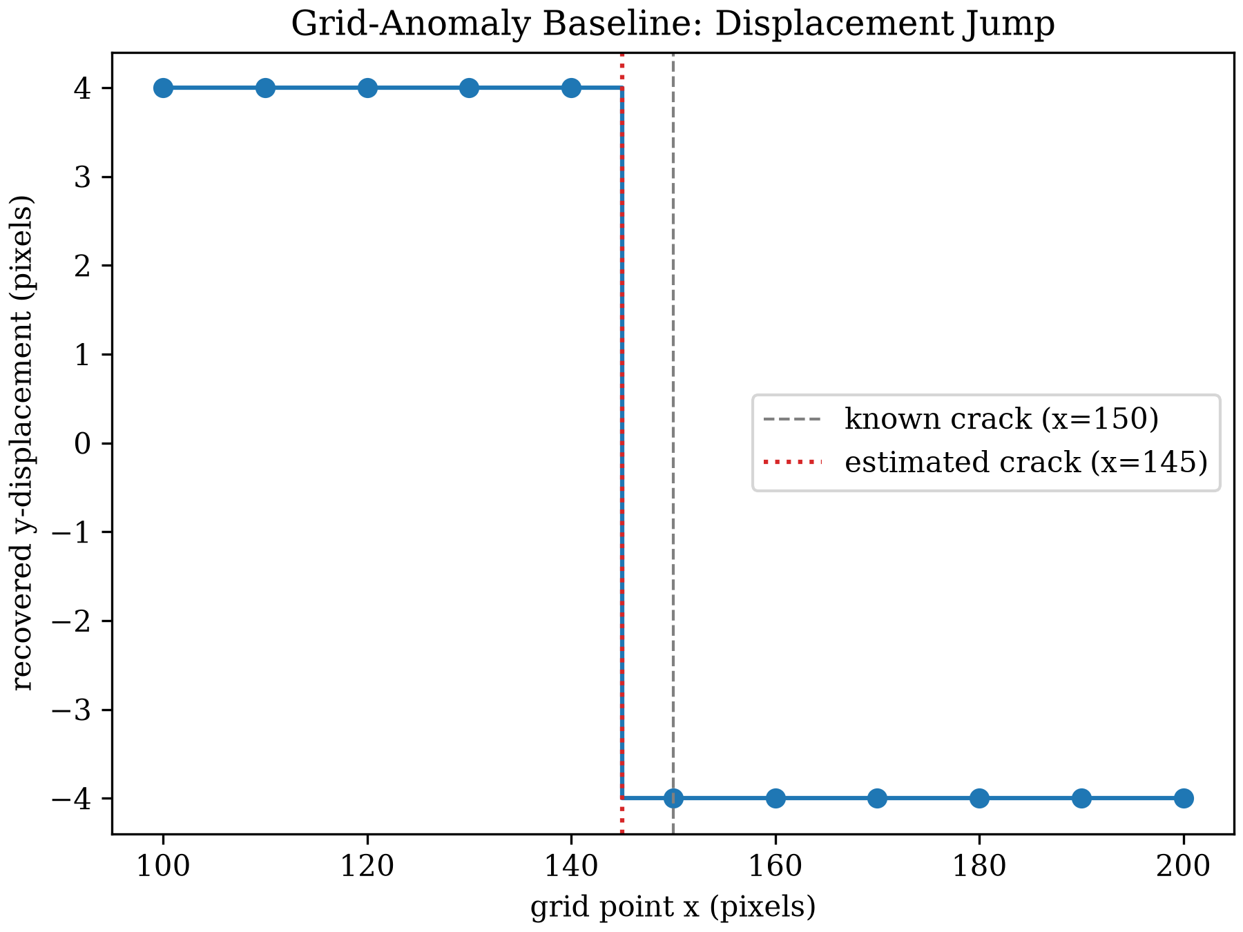
step plot of recovered y-displacement vs grid point x: a flat line at +4 pixels for x=100 through 140, then a sharp step down to -4 pixels for x=150 through 200, with the estimated crossing at x=145 marked slightly left of the true crack at x=150 — Recovered y-displacement at 11 grid points, spaced 10 pixels apart. The jump between x=140 and x=150 is unmistakable: +4 pixels on one side, -4 on the other. The midpoint between them, x=145, lands 5 pixels from the true crack at x=150. That's half the grid spacing: exactly the resolution this approach can offer, no better.

It works, in the sense that it flags roughly the right neighborhood. It's also a proxy, not a measurement of the thing itself. Nothing here looks at peak structure. A large stretch, not a crack, would produce the same kind of jump. Resolution is capped at the grid's own spacing. Tighten the grid and the jump narrows, but so does how many points a DIC run at that spacing can afford to place.

A Peak-Ratio Metric

Synthetic Dislocation already measured a straddling window's two peaks by hand: heights 0.528 and 0.519 at x=150. Turning that into a number that needs no ground truth: dictk.discontinuity.peak_ratio divides the second-tallest peak by the tallest, along the correlation surface's own argmax column.

from dictk.correlation import zncc
from dictk.discontinuity import peak_ratio
from dictk.image import PixelCoordinate, subimage

for x in (150, 100):
    p0 = PixelCoordinate(x=x, y=150)
    kernel = subimage(
        image=reference_image,
        origin=PixelCoordinate(x=p0.x - 25, y=p0.y - 25),
        width=50, height=50,
    )
    search = subimage(
        image=current_image,
        origin=PixelCoordinate(x=p0.x - 45, y=p0.y - 45),
        width=90, height=90,
    )
    ratio = peak_ratio(surface=zncc(kernel=kernel, search=search))
    print(f"x={x}: peak_ratio={ratio:.3f}")

x=150: peak_ratio=0.983
x=100: peak_ratio=0.000

Centered on the crack, peak_ratio is 0.983, close to the 1.0 two perfectly equal peaks would give. At x=100, well clear of the crack, it's 0.0: one peak resolvable, nothing to divide against. A single number now stands in for "does this window straddle a discontinuity," with no offset to already know in advance.

dictk.discontinuity.sweep evaluates peak_ratio at many window-center positions along a line, and dictk.discontinuity.locate takes that sweep's tallest value and refines it to subpixel precision with a 3-point parabolic fit. Sweeping the same x=100 to x=200 range Synthetic Dislocation already swept by hand:

Evaluations: 101 Located crack position: x=149.804 Error vs. known x=150: 0.196px

Saved: discontinuity_localization_sweep.png

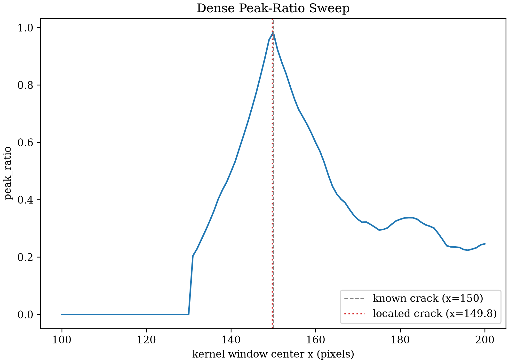
line plot of peak_ratio vs window center x from 100 to 200, rising from 0 at x=130 to a sharp peak near 1.0 at x=150, then falling and settling into a fluctuating 0.2-0.3 band past x=170 — peak_ratio vs. window center x. A single, sharp maximum at x=149.8, subpixel-refined from a 101-point sweep. The known crack sits at x=150, 0.2 pixels away. Past x=170, peak_ratio settles into the same 0.2-0.3 band Synthetic Dislocation's own sweep already found and attributed to the underlying image content on that side, not the crack.

101 evaluations, one per swept position, land 0.2 pixels from the known crack. No offset, no hand-picked center. The sweep finds the crossing on its own.

A Faster Alternative: Golden-Section Search

A dense sweep evaluates every candidate position, even the ones far from any discontinuity. peak_ratio rises to a single maximum and falls away on both sides of the crack. That's exactly the shape a derivative-free optimizer can search without visiting every point. Golden-section search narrows a bracket toward a unimodal function's maximum in $O (lo g n)$ evaluations instead of sweep's $O (n)$ :

Golden-section result: x=150.25, evaluations=12 Error vs. known x=150: 0.251px

Approach	Evaluations	Localization Error (px)	Notes
Grid anomaly (baseline)	11	5.0	resolution capped at 10px grid spacing
Dense peak-ratio sweep (winner)	101	0.196	robust to bracket width, see below
Golden-section peak-ratio search	12	0.251	fast here, breaks on real data -- see below

Saved: discontinuity_localization_bisection.png

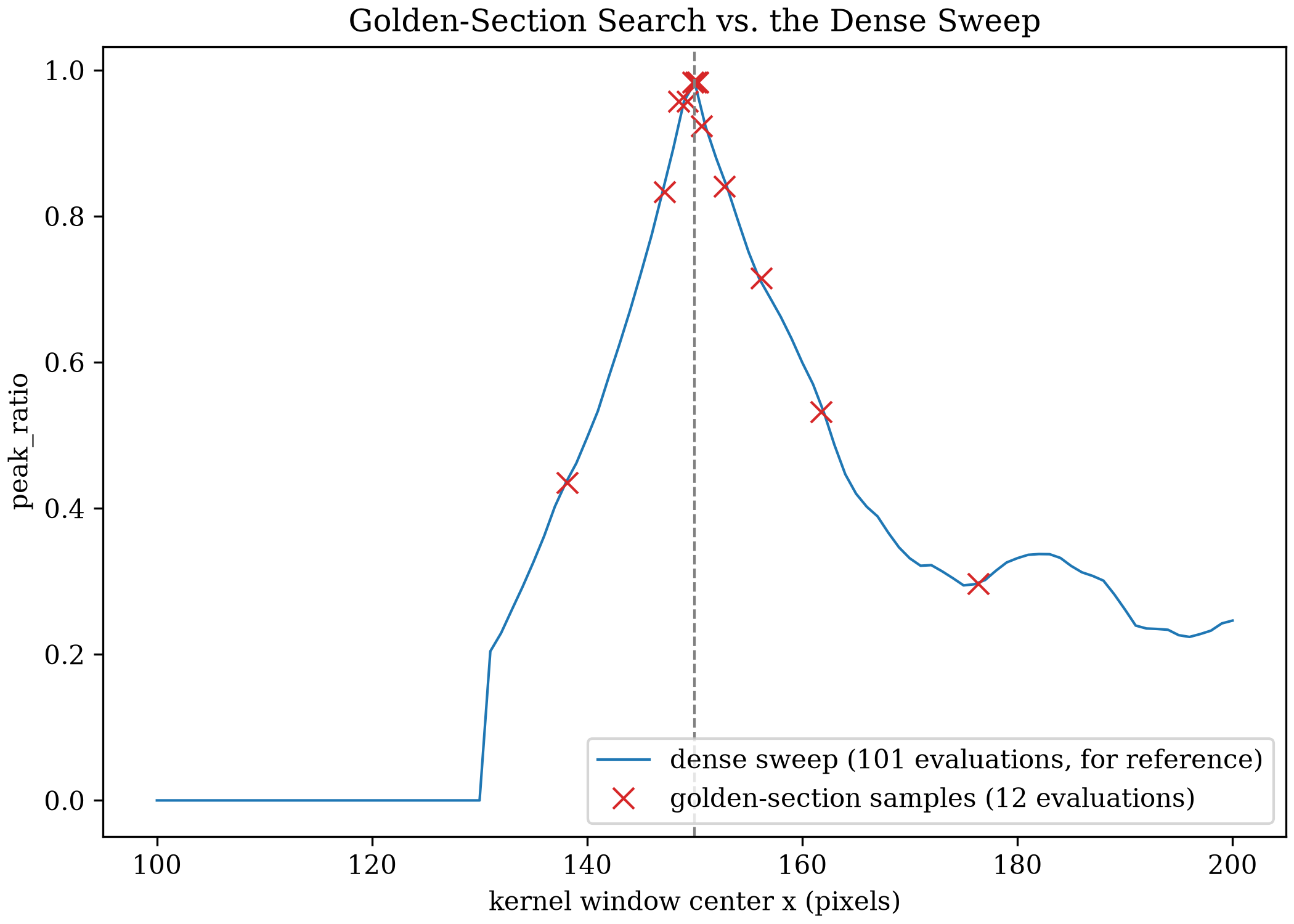
the same peak_ratio curve as the dense sweep figure, with red x markers showing golden-section search's 12 sampled points clustered tightly around the true peak at x=150 — Golden-section search's own 12 sampled points, against the dense sweep's full curve for reference. All 12 cluster near the true maximum. The search needed no help finding it.

12 evaluations instead of 101, landing 0.25 pixels from the known crack. That's barely worse than the dense sweep, for roughly a tenth of the cost. On this dataset, it looks like a strictly better trade.

Applying It to Real Data

Experimental Dislocation already centered a window by eye on the real crack, at x=218, y=186. This runs the dense sweep across a much wider range, x=100 to x=350, assuming nothing about roughly where the crack sits. It also runs golden-section search at three brackets: one already centered tightly on the crack, one moderately wide, and one as wide as the dense sweep's own range.

Dense sweep (wide range 100-350, 126 evaluations): located crack position: x=218.74 (Experimental Dislocation's own x=218)

golden-section, bracket (178, 258): x=217.55, evaluations=12 golden-section, bracket (150, 300): x=217.25, evaluations=13 golden-section, bracket (100, 350): x=308.11, evaluations=14

The tight and moderate brackets land within 1px of the dense sweep's own answer. The wide bracket -- the one that assumes no prior knowledge of roughly where the crack is -- converges instead to a smaller, secondary peak_ratio bump far from the real crack, confidently and silently. Saved: discontinuity_localization_experimental.png

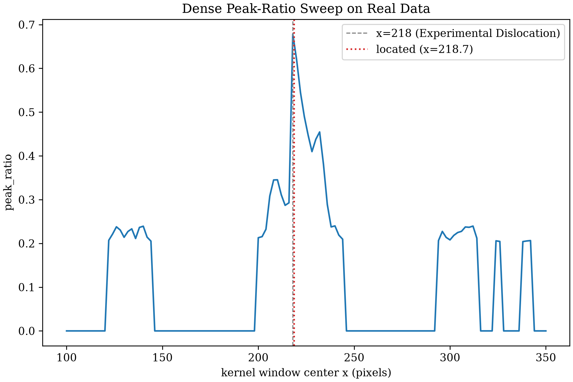
line plot of peak_ratio vs window center x from 100 to 350 on real data: a tall sharp peak near x=219, plus three smaller, shorter bumps around x=130, x=300-315, and x=325-340 — peak_ratio across a wide real-data range. One peak clearly stands above the rest, at x=218.7, 0.7 pixels from Experimental Dislocation's own by-eye x=218. Three smaller bumps sit elsewhere in the image, each shorter than the real crack's peak, but not by a wide margin.

The dense sweep's global maximum lands within a pixel of the known location, no matter how wide a range it searches. Golden-section search does too, but only at the two brackets already narrowed toward the crack. Given the full, uncommitted range, it converges instead to the bump near x=308, over 90 pixels from the real crack, confidently and silently. A fast local search only works once you already roughly know where to look. That's most of the problem this page set out to solve in the first place.

Declaring a Winner

The dense sweep, with subpixel parabolic refinement, ships as dictk.discontinuity. It needs no prior estimate of where a crack sits, its accuracy doesn't depend on how wide a range it searches, and it holds up on both synthetic and real data. The grid-anomaly baseline and golden-section search stay as illustrations on this page, not library code: the baseline only ever offers grid-spacing resolution, and golden-section search's speed comes at the cost of needing the answer roughly in hand before it can find it.

Approach	Evaluations (synthetic)	Localization Error (synthetic)	Real Data
Grid anomaly (baseline)	11	5.0 px	weaker, noisier jump signal
Dense peak-ratio sweep (winner)	101	0.2 px	0.7 px from by-eye estimate
Golden-section search	12	0.25 px	fails on a wide, honest bracket

What This Still Doesn't Do

This locates a crossing along one already-chosen line, not a discontinuity anywhere in a 2D field. Something still has to decide where to sweep. And a located position still isn't consumed by anything: Path Forward's Heaviside DIC/XFEM item asked for detection and localization, not a finite-element formulation that acts on the result. That half stays open.

Continue to Path Forward for where this leaves it.